
What it is
It turns text into vectors, and a head you train turns those into answers
An encoder takes a piece of text and gives you back one vector for every token in it. A token is a word or a piece of a word, and a vector is a list of numbers describing that token in the context of everything around it. Those vectors don't answer anything by themselves. To get an answer out of the model you attach a head, which is a small output layer with one slot for each of your labels, and you train that head on examples of the decision you want it to make.
BERT also puts a special [CLS] token in front of every input you hand it. The paper calls the final vector at that position "the aggregate sequence representation for classification tasks", which is a formal way of saying that one vector stands for the whole piece of text. If you are classifying, your head reads that single vector and picks a label. If you are pulling pieces out of a sentence, say every date in a contract, your head reads every token's vector and labels each one separately.
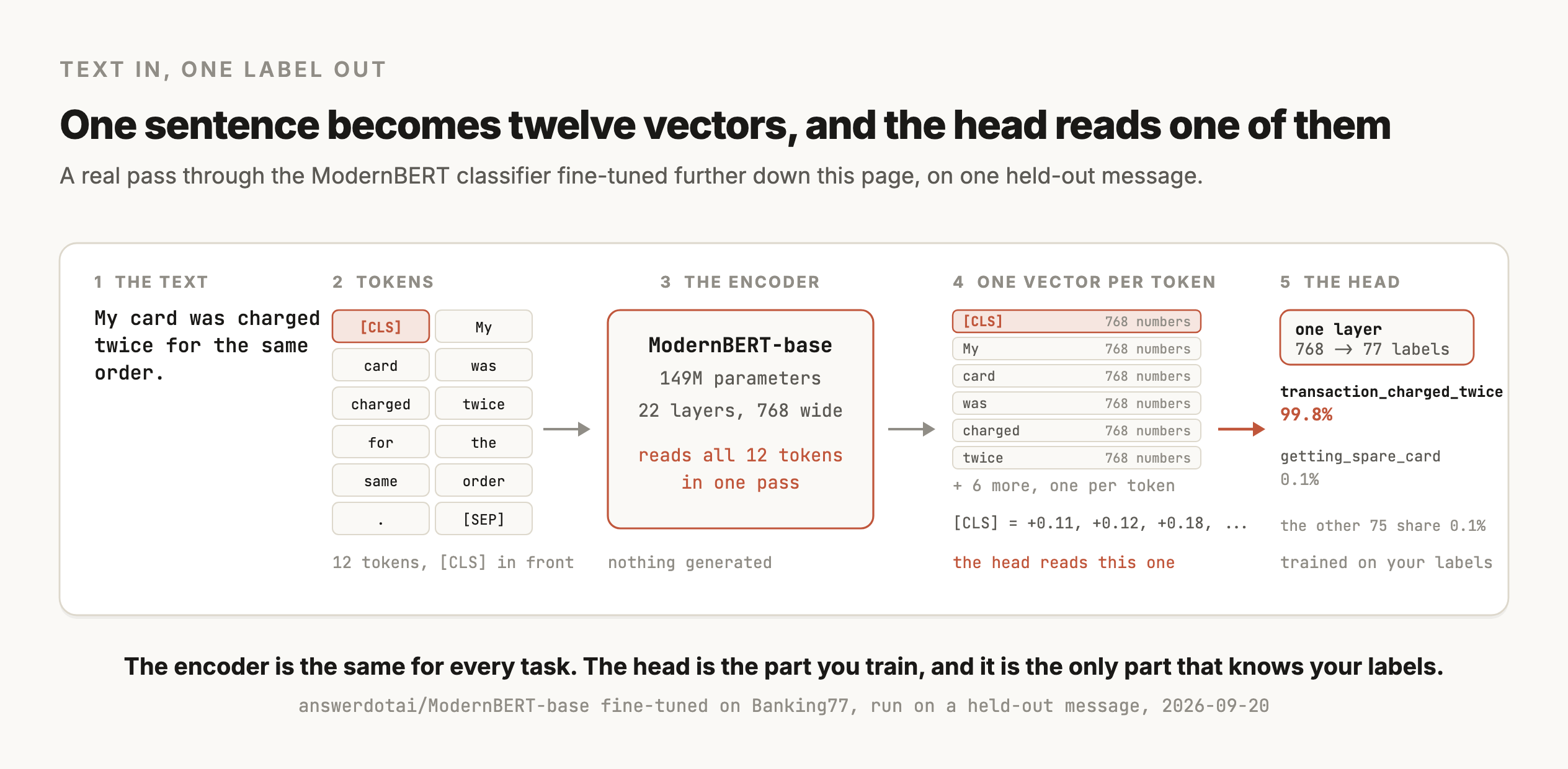
Every position reads the whole input in both directions, so by the time the model judges a word it has already read the words that come after it. The word charge means one thing in "they charged my card twice" and a different thing in "the battery will not charge", and an encoder has read the rest of the sentence before it settles on either one. The encoder, decoder and encoder-decoder article draws that out with a figure, if you want to see the mechanism.
Where it shows up
Encoders do the small jobs that run on every record
Classifying text into labels you already have examples of
This is the job the model was built for. You have a few thousand support tickets that somebody already routed, or a pile of reviews somebody already scored, and you want the same decision made on every new one that arrives. The labels stay the same from week to week, and the model runs on every single record. The measured run further down this page is exactly this job.
Pulling the pieces out of a sentence
Named entity recognition, usually written as NER, puts a label on each token, so one pass through a contract marks every person and every date in it. GLiNER takes that further by letting you name the entity types you care about at request time, because it puts those type names into the input right next to the text.
Reranking search results
A cross-encoder reads the query and one document together, in the same input, and gives you a score for that pair. Reading them together is what makes it accurate, and it also means nothing can be computed ahead of time, so it only runs on the shortlist that a faster search step already returned. The design goes back to monoBERT in 2019.
Producing embeddings
Most text embedding models are encoders with a pooling step on the end, which usually means averaging the token vectors into a single vector for the whole document. Search and deduplication over your own content both start there.
Guardrails in front of an LLM
Prompt injection detection, which is checking whether the user's text is trying to override the instructions you gave the model, has to run on every single request, so the model doing the checking needs to be small and fast. protectai/deberta-v3-base-prompt-injection-v2 is a 184M encoder that returns the probability that an input is an injection attempt, and it gets about 850,000 downloads a month.
Turning a pile of text into columns you can chart
Running a fine-tuned classifier over a few million rows is cheap enough to put on a schedule and let it run overnight. Every review comes back with a topic and a sentiment attached, and free text you could only read becomes a column you can sort, filter and chart.
How it works
Mask words to pretrain it, then add a head to fine-tune it
Pretraining masks words and asks for them back
BERT masks 15% of the tokens in each sequence and tries to predict them, reading both sides of every gap. Hand ModernBERT the sentence "They [MASK] my card twice for the same order" and it answers charged at 33.5%, used at 8.7% and sent at 3.3%, working only from the words around the hole.
It can't be trained to predict the next word the way an LLM is, because a model that reads in both directions has already seen that word. The paper puts it as "bidirectional conditioning would allow each word to indirectly see itself". Masking gives it something to predict that it can't already see.
Later encoders changed parts of this. RoBERTa trained for longer on more data and dropped BERT's second training objective, which had asked the model whether two sentences followed each other in the original document. DeBERTaV3 swapped masked language modeling for replaced token detection, where the model looks at every token and decides whether it is the original word or a substitute that was slipped in. Every position in the sequence carries a training signal that way, which the paper describes as a more sample-efficient task.
Fine-tuning attaches your head and moves every weight
You load the pretrained encoder, attach a fresh output layer with one slot per label, and train on your labeled examples. The head starts out random, so at the first step it is guessing. Every other weight in the model starts pretrained and keeps moving while you train, which is why a few thousand examples are usually enough.
from transformers import AutoModelForSequenceClassification, AutoTokenizer

model_id = "answerdotai/ModernBERT-base"
tok = AutoTokenizer.from_pretrained(model_id)
model = AutoModelForSequenceClassification.from_pretrained(
    model_id, num_labels=77)                   # 77 output slots, randomly set

batch = tok(texts, padding="max_length", truncation=True,
            max_length=64, return_tensors="pt")
batch["labels"] = label_ids                    # one integer per example
loss = model(**batch).loss                     # backward, step, repeat
What a modern encoder changed
ModernBERT came out in December 2024, and it is the same design with eight years of newer engineering applied to it. It was trained on 2 trillion tokens and it reads up to 8,192 tokens at a time, where the original BERT stopped at 512. Its layers alternate between global attention, where every token reads every other one, and a 128-token sliding window, and the paper says "every third layer" does the global pass. It also strips out padding tokens, which are the filler added to short inputs so every row in a batch is the same length, so the model computes only on real words. The result is a 149M and a 395M model that process long sequences about twice as fast as the encoders before them.
A measured run on 13,083 real messages
Banking77 is a public dataset from Casanueva et al. (2020). It holds 13,083 real messages that customers sent to a bank, each one labeled with one of 77 intents, and it comes already split into 10,003 messages for training and 3,080 for testing. It stands in well for the kind of work people put a classifier on, because 77 labels is more than a prompt handles comfortably and a lot of those intents sit close to each other.
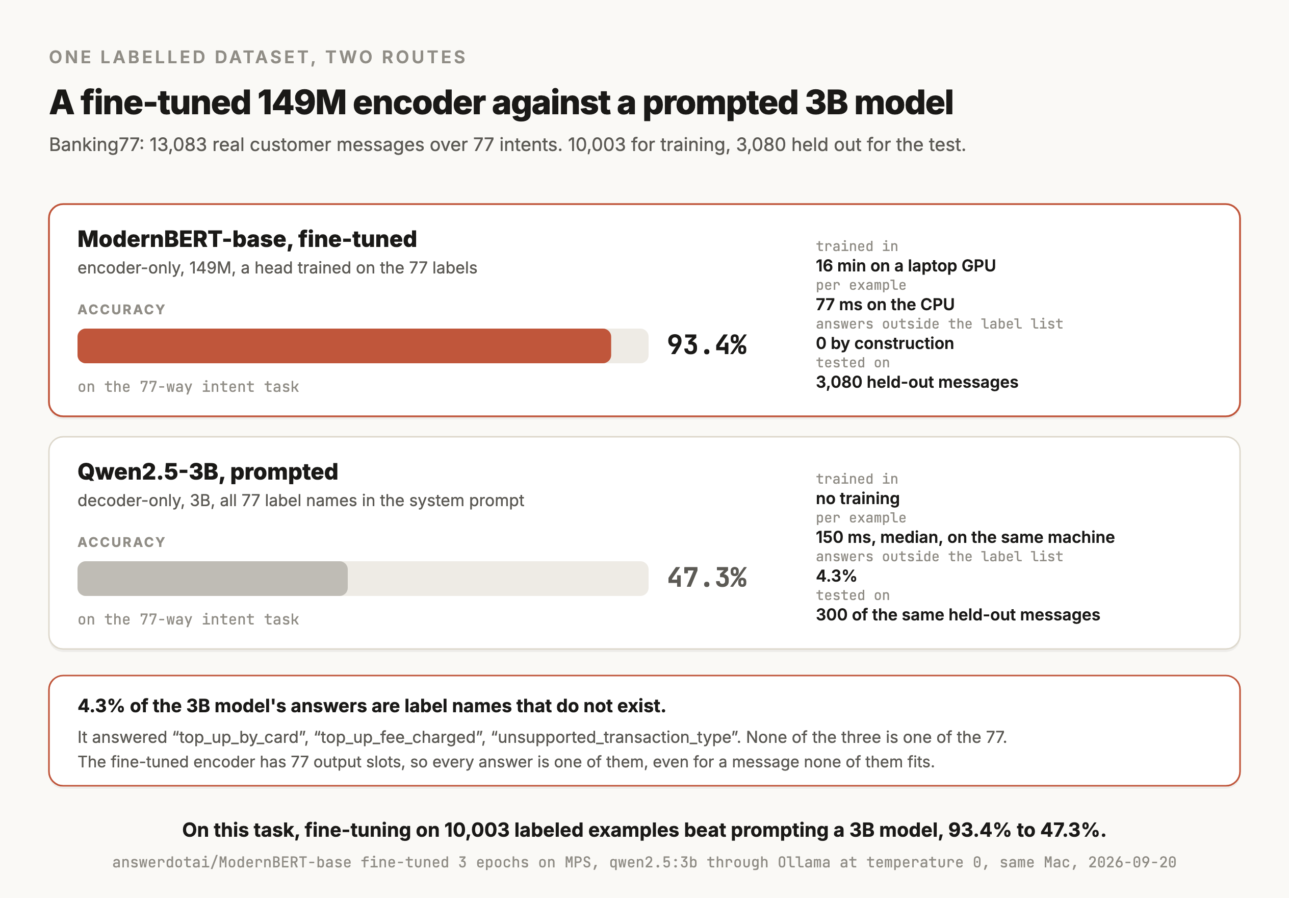
Fine-tuning ModernBERT-base for three epochs took 15.6 minutes on the laptop's GPU, and it got 93.4% of the 3,080 held-out messages right. Prompting Qwen2.5-3B with all 77 label names in the system prompt, on 300 of those same messages, got 47.3%. Once it is trained, the encoder answers in 77 milliseconds on the CPU, with no GPU and no API call involved.
That figure is about this one task and these two models. A bigger prompted model would probably score higher than 47.3%, and this run didn't test one, so it can't say whether a larger model or a frontier model prompted with the same 77 labels would pass 93.4%. What the run does show is that 10,003 labeled examples took a 149M model to 93.4% on this task, and that the model runs on hardware you already own.
The two models also fail in different ways. 4.3% of the 3B model's answers were label names that do not exist, assembled out of the ones that do, like top_up_by_card when the real label is topping_up_by_card. A fine-tuned encoder has exactly 77 output slots, so there is nothing else it could return. Every mistake it makes on these test messages is a confusion between two real labels, which you can find in a confusion matrix and fix by labeling more examples of the pairs it keeps mixing up.
The same 77 slots mean it can't say "none of these". The softmax spreads all of its probability across the 77 intents, so a message about something no intent covers, like a question about the weather, still comes back as one of them. Banking77's test messages all belong to one of the 77 intents, so this run doesn't measure how often that happens. The usual fixes are an extra other label trained on real off-topic messages, and a threshold on the top probability that sends low answers to a person. Hendrycks and Gimpel (2017) found that "correctly classified examples tend to have greater maximum softmax probabilities than erroneously classified and out-of-distribution examples", which is why that threshold catches some of them. The tendency is an average, so some off-topic messages still get a high probability.
Versions
These are the checkpoints you'll see, as of September 2026
| Model | Released | Size | License | Downloads a month |
|---|---|---|---|---|
google-bert/bert-base-uncased | October 2018 | 110M | Apache-2.0 | 46.6M |
FacebookAI/roberta-base | July 2019 | 125M | MIT | 7.9M |
distilbert/distilbert-base-uncased | October 2019 | 66M | Apache-2.0 | 7.6M |
microsoft/deberta-v3-base | November 2021 | 184M | MIT | 2.9M |
answerdotai/ModernBERT-base | December 2024 | 149M | Apache-2.0 | 4.4M |
answerdotai/ModernBERT-large | December 2024 | 395M | Apache-2.0 | 0.6M |
jhu-clsp/mmBERT-base | September 2025 | 307M, 110M without embeddings | MIT | 0.4M |
ModernBERT is what to start from for new work in English, since it reads 8,192 tokens at a time and carries an Apache-2.0 license. mmBERT is the multilingual one, pretrained on 3 trillion tokens covering over 1,800 languages, so reach for it when the text you are working with is not in English.
The models running in production today are years old. A fine-tuned encoder keeps doing its job, and moving to a newer one costs a retraining run, so it's worth doing when a test on your own held-out data shows a gain.
Choosing
Choose an encoder when the labels are fixed and the volume is high
| The job | Reach for | Why |
|---|---|---|
| Classify into fixed labels you have examples of | A fine-tuned encoder | The accuracy comes from your labels, and the model is small enough to run anywhere |
| Classify with no labeled data | An LLM with the categories in the prompt, or Jev | Nothing to train, and you can change the categories in the request |
| Labels that change every week | An LLM or Jev | A new label means a new request, where an encoder means retraining |
| High volume with stable labels | A fine-tuned encoder | A 149M model on your own hardware costs a fraction of an API call |
| Data that can't leave your network | A fine-tuned encoder | Open weights that run on your own CPU, with nothing sent anywhere |
| Write a reply or a summary | An LLM | An encoder produces vectors and can't write |
| Rank documents for a query | A cross-encoder reranker | It reads the query and the document together |
| Find similar text | An embedding model | One vector per document, compared by cosine similarity |
If you are starting from nothing, the order that usually works is to prompt a model first and fine-tune an encoder later, once the volume is high enough for the cost to show up on a bill or the accuracy stops being good enough. The prompting stage is also how you get your labeled examples, because a good LLM's output, corrected by a person, is a labeled dataset.
Try it
How to try it
Before you point any of this at your own data, it is worth running it once on a public dataset so you know the pipeline works end to end. This script loads the dataset from the figure above and trains the classifier on it.
import torch
from datasets import load_dataset
from transformers import (AutoModelForSequenceClassification, AutoTokenizer,
                          Trainer, TrainingArguments)

ds = load_dataset("PolyAI/banking77")          # 10,003 train, 3,080 test
labels = ds["train"].features["label"].names   # 77 intents

model_id = "answerdotai/ModernBERT-base"
tok = AutoTokenizer.from_pretrained(model_id)
model = AutoModelForSequenceClassification.from_pretrained(
    model_id, num_labels=len(labels))

enc = ds.map(lambda b: tok(b["text"], truncation=True, max_length=64),
             batched=True)

Trainer(model=model, train_dataset=enc["train"], eval_dataset=enc["test"],
        args=TrainingArguments(output_dir="out", num_train_epochs=3,
                               per_device_train_batch_size=32,
                               learning_rate=5e-5)).train()
On a laptop GPU this finishes in about 16 minutes. When you swap in your own CSV, nothing else in the file has to change.
Fine-tune an encoder on my labeled text and tell me whether it's good enough to ship. Read data.csv with text and label columns, hold out 20% stratified by label, and fine-tune answerdotai/ModernBERT-base with AutoModelForSequenceClassification for 3 epochs. Report accuracy and macro F1 overall and per label, and save a confusion matrix as a PNG with the 10 most-confused label pairs listed underneath. Then run a learning-curve experiment that retrains on 10%, 25%, 50% and 100% of the training rows and plots accuracy against the number of examples, so I can see whether more labeling would help. Finally, measure median and p95 latency per example on CPU at batch size 1 and at batch size 32.
Limits
What it can't do
- It can't write anything. There is no way to get a summary or a written reply out of it, because every answer it produces is a label or a score coming out of the head you trained.
- It can't reject an input that fits none of its labels. Every input gets one of the labels you trained, so an off-topic message needs an
otherlabel of its own or a threshold on the probability to be caught. - Its labels are fixed the moment you train it. Adding a category means collecting new examples and running training again, where a prompted model takes the new category in the request.
- It needs labeled data. A few dozen examples per label is the rough floor, and the accuracy in the figure came from about 130 examples per intent.
- Its probabilities need checking before you put a threshold on them. The head's scores are turned into percentages by a softmax, and a 0.92 there does not mean the model is right 92% of the time. The usual fix is temperature scaling, which is one number, fitted on held-out examples, that flattens or sharpens every probability at once.
- Long inputs are still a constraint. Older encoders stop at 512 tokens, so a long document has to be split into chunks first. ModernBERT's 8,192 is recent enough that most of the fine-tuning recipes you will find online still assume the old limit.
- It carries whatever was in its pretraining data. The English checkpoints were trained on web text, and the biases and blind spots that came with that text survive fine-tuning.
Go deeper
Devlin et al. (2018): BERT, Pre-training of Deep Bidirectional Transformers for Language Understanding · Liu et al. (2019): RoBERTa, A Robustly Optimized BERT Pretraining Approach · He et al. (2021): DeBERTaV3, ELECTRA-Style Pre-Training with Gradient-Disentangled Embedding Sharing · Warner et al. (2024): ModernBERT, a modern bidirectional encoder · Marone et al. (2025): mmBERT, a modern multilingual encoder · Casanueva et al. (2020): Efficient Intent Detection with Dual Sentence Encoders (the Banking77 dataset) · Stepanov et al. (2025): GLiClass, a generalist lightweight model for sequence classification
Coming soon
New modules go live as I write them. Get each one in your inbox the day it ships. No spam, just the next lesson.