
What it is
The query is present, or it isn't
A bi-encoder runs the encoder twice, once over each text, and compares the two vectors it gets back. The document half runs once when you build your index, and the query half runs when somebody searches. Everything about its speed follows from the document vector existing before the query does.
A cross-encoder runs the encoder once over both texts joined into a single input, with a separator between them, and reads a score off the end. Every layer of the model can look from a word in the query to a word in the document, which is the accuracy, and the score exists only for that one pair, which is the cost.
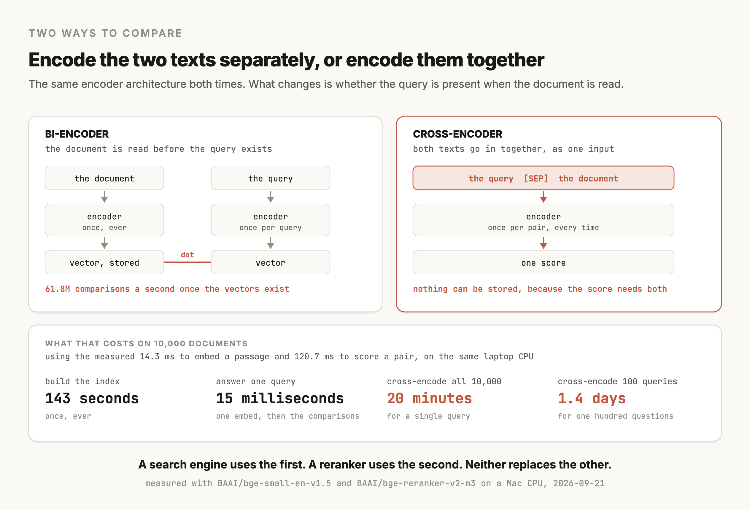
The numbers in that strip are the argument. Building a searchable index of 10,000 passages took 143 seconds once. Answering a query off that index took 15 milliseconds. Scoring the same 10,000 passages with a cross-encoder takes 20 minutes, for one question, every time it is asked.
All of those are sequential timings, one text or one pair at a time on a laptop CPU, which is how the 120.7 ms per pair was measured. A real reranker sends pairs through the model in batches, and on a GPU a batch of dozens of pairs usually takes only a little longer than a single pair, so the 20 minutes could shrink a lot. This page didn't measure a batched run, so treat the size of that drop as something to time on your own hardware. What batching can't change is that the work still grows with the number of documents scored for every query, because each pair is a full pass through the model. The bi-encoder's per-query work stays at one embedding and a cheap comparison whatever the collection size, so batching narrows the gap between the two designs without removing it.
Which models use this
Which models are which
| Design | Models | What it is used for |
|---|---|---|
| Bi-encoder | Text embedding models such as bge, E5 and Qwen3-Embedding | Search, clustering, deduplication |
| Bi-encoder | CLIP and SigLIP, with one tower for images and one for text | Image search and zero-shot classification |
| Bi-encoder | Two-tower retrieval models in recommendation systems | Picking a few hundred candidates out of millions of items |
| Cross-encoder | Rerankers such as bge-reranker and Cohere Rerank | Rescoring a shortlist |
| Cross-encoder | Natural language inference models, which judge whether one sentence follows from another | Fact checking and contradiction detection |
| Cross-encoder | Jev and the classifiers that read a document and a question together | Typed decisions over one piece of text |
CLIP makes that trade most visibly. Its two towers never see each other's input, which is exactly why you can embed a million photos once and then search them with any sentence you type. The price is the one the CLIP article measures, where the raw scores sit in a narrow band and mean little on their own.
How it works
What reading together buys, and what it costs
The bi-encoder has to guess what you will ask
A document vector has to be useful for every question anyone might ask of that document, because it is computed before any of them arrive. It is a summary with no idea what it will be asked.
That is why two passages about training on labelled data end up near each other even when one is about images and the other about text. The distinction was never in the question when the vector was made.
The cross-encoder is told what you asked
With both texts in one input, attention can run between them at every layer. The model can check the specific words of your question against the specific words of the passage, which is how the rerankers run separates "labelled examples" in a question about text from "labeled images" in a passage about object detection.
The measured gain on that run was 4 of 8 questions answered from the right article becoming 6 of 8, on the same corpus, with the same first stage.
Precomputation is the whole difference
The bi-encoder's document pass depends on nothing but the document, so its result can be stored and reused forever, for every query anyone asks. The cross-encoder has no query-independent step to store. Every layer mixes query tokens with document tokens, so even the document's first-layer vectors change when the query changes.
A cross-encoder's output can still be cached, but only as a score for one exact pair. If the same query comes back against the same passage, a cache keyed on both texts returns the old score without running the model. That helps with repeated popular queries, and it does nothing for a query that differs by one word, since that is a new pair. A cache like that can't be indexed or searched either, because each score belongs to a single query.
This is also why a bi-encoder comparison is nearly free. Once both vectors exist, comparing them is a dot product, and a million of those took 16 milliseconds on the machine behind the figure.
ColBERT sits between the two
Khattab and Zaharia (2020) built ColBERT on a third arrangement. It runs the encoder over the document ahead of time the way a bi-encoder does, and it keeps the vector for every token rather than pooling them into one. At query time it does the same for the query, then compares the two sets of vectors token by token, which the paper calls late interaction.
The comparison itself is called MaxSim. Every query vector finds the closest vector in the passage, that one similarity is kept, and the kept scores are added up to give the passage its score. Running it on the question the embedding model got wrong shows both the mechanism and a piece of ColBERT that is easy to miss.
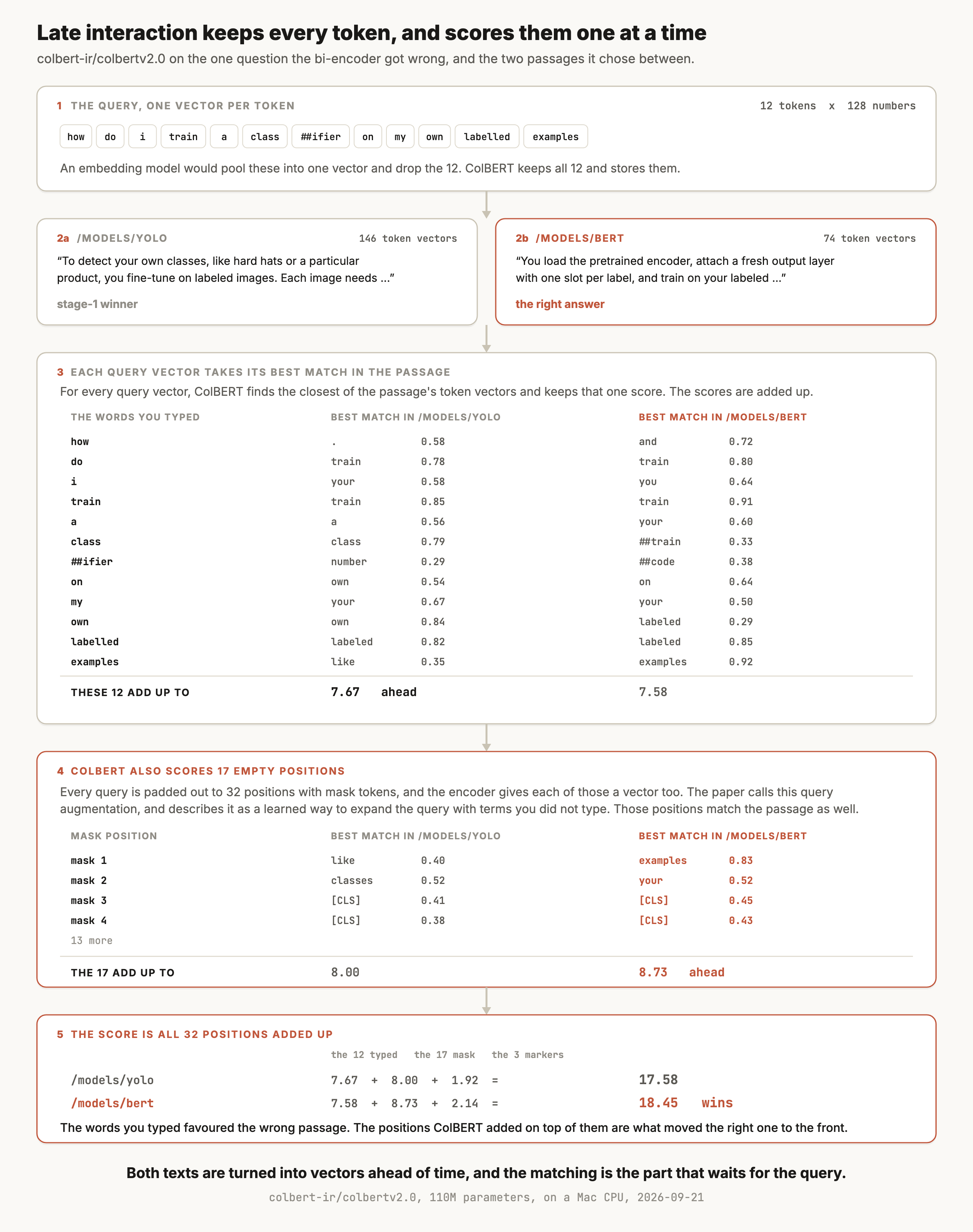
Two things in that run are worth taking away. The first is that word-level matching does what you would expect, and "examples" in the question finds the word examples in the BERT passage at 0.92 while finding nothing better than "like" in the YOLO one at 0.35.
The second is that the typed words alone still put the wrong passage first, at 7.67 against 7.58. What moved the right passage to the front was the 17 mask positions ColBERT pads every query with. The paper describes that padding as "a soft, differentiable mechanism for learning to expand queries with new terms or to re-weigh existing terms", and on this pair it contributed more of the score than the question did.
The trade is index size. A passage that cost one vector now costs one per token, so the 287 passages behind these figures would go from 287 vectors to tens of thousands. ColBERT's own later work spends most of its effort on compressing exactly that.
Choosing
Choosing, which usually means using both
| The step | Design | Why |
|---|---|---|
| Finding candidates in a large collection | Bi-encoder | The document vectors already exist, so the search is a comparison |
| Reordering the top 10 to 50 | Cross-encoder | It reads the pair, and the shortlist is small enough to afford it |
| Comparing two fixed texts, one pair at a time | Cross-encoder | No index is involved, so nothing is gained by precomputing |
| Clustering or deduplicating a collection | Bi-encoder | Vectors can be compared with each other, and pair scores cannot |
| Matching text against images | A bi-encoder such as CLIP | Two towers is what makes a searchable image index possible |
| Deciding one yes-or-no about one document | Cross-encoder, or Jev | Both read the pair and return a score you can threshold |
The usual answer is both, in that order. Retrieve with the bi-encoder, rerank the top of it with the cross-encoder, and choose the shortlist depth by measuring how often the right answer appears in it. That structure is why the text embeddings and rerankers articles use the same corpus and the same eight questions.
Try it
How to try it
Both designs are a few lines in transformers, and running them side by side on your own pairs is the fastest way to feel the difference.
import torch
from transformers import (AutoModel, AutoModelForSequenceClassification,
                          AutoTokenizer)

query, doc = "how do I train a classifier", "You load the pretrained encoder..."

# bi-encoder: two passes, and the document half is reusable
bt = AutoTokenizer.from_pretrained("BAAI/bge-small-en-v1.5")
bm = AutoModel.from_pretrained("BAAI/bge-small-en-v1.5").eval()
def vec(text):
    with torch.no_grad():
        h = bm(**bt(text, return_tensors="pt")).last_hidden_state[:, 0]
    return torch.nn.functional.normalize(h, dim=-1)
print("cosine:", float(vec(query) @ vec(doc).T))

# cross-encoder: one pass over both, and nothing is reusable
ct = AutoTokenizer.from_pretrained("BAAI/bge-reranker-v2-m3")
cm = AutoModelForSequenceClassification.from_pretrained(
    "BAAI/bge-reranker-v2-m3").eval()
with torch.no_grad():
    print("score:", float(cm(**ct([[query, doc]],
          return_tensors="pt")).logits))
The two numbers are on different scales and are not comparable. The cosine sits in a narrow band across all pairs, and the cross-encoder score spreads out, which is the practical reason one sorts well and the other thresholds well.
Show me the speed and accuracy trade between the two designs on my own data. Take a CSV of query and document pairs with a relevance label. Score every pair two ways, once with BAAI/bge-small-en-v1.5 as a bi-encoder using cosine similarity, and once with BAAI/bge-reranker-v2-m3 as a cross-encoder. Report the area under the ROC curve for each. Time the cross-encoder twice, once scoring pairs one at a time and once in batches of 32, and time the bi-encoder's document embedding separately from its query embedding, since the documents only need embedding once. Then estimate how long each design would take to answer one new query against 10,000 documents, counting only the work that has to happen after the query arrives. Then plot both score distributions for relevant and irrelevant pairs on one chart, so I can see which of the two has a usable threshold.
Limits
What neither design fixes
- A bi-encoder cannot recover a distinction it was never told about. The document vector is made before the query exists, so a question that turns on a detail the summary dropped cannot be answered by better comparison.
- A cross-encoder cannot search. Scoring every document for every query is the 20 minutes in the figure when run one pair at a time, and batching on a GPU cuts that time without changing how the work grows with the collection, so it always depends on something else handing it a shortlist.
- Neither score is calibrated out of the box. A cosine sits in a narrow band, and a cross-encoder logit is on no fixed scale, so any threshold has to be fitted on your own labelled pairs.
- Both truncate. A bi-encoder truncates the document to its context limit, and a cross-encoder splits that limit between the query and the document, so long passages lose their tails either way.
- The accuracy gap depends on your corpus. The measured gain behind these pages was two questions out of eight on one small corpus, and on a corpus where retrieval already ranks well, a reranker adds latency and little else.
Go deeper
Reimers and Gurevych (2019): Sentence-BERT, Sentence Embeddings using Siamese BERT-Networks · Nogueira and Cho (2019): Passage Re-ranking with BERT · Khattab and Zaharia (2020): ColBERT, Efficient and Effective Passage Search via Contextualized Late Interaction · Devlin et al. (2018): BERT, the encoder both designs are built on
Coming soon
New modules go live as I write them. Get each one in your inbox the day it ships. No spam, just the next lesson.