
The capability
What retrieval-augmented generation is
As you already know from M3, when a model answers, all it has to go on is what it learned in training and the text you put in the request. It has never seen your company's parental leave policy or the fault codes in your robot manuals, so if you ask it about them it will either say it doesn't know or, more often, write something that sounds right. Retrieval-augmented generation, RAG for short, is how you get those documents in front of it. When a question comes in, your code searches your documents for the passages that bear on it, puts those passages into the request next to the question, and asks the model to answer from them and say which passage each claim came from.
So a RAG system has two parts. One is a search system, which has to find the right few passages out of thousands of documents in a fraction of a second, for this particular person, from the current version of each document. For search by meaning, that usually means turning every passage into an embedding, a list of numbers that captures what it's about, and storing those in a vector database that can find the embeddings closest to the question's. Search by keyword works too, and section 11 shows why good systems run both. The other is the model call M4 and M5 already covered, now with a stricter job, because it has to answer from the passages it was given and say so when they don't contain the answer. Most of the engineering in this module is on the search side, because a model can't answer from a passage that never reached it.
The name comes from a 2020 paper by Lewis and colleagues at Facebook AI Research, which paired a BART generator with a neural retriever over Wikipedia split into 100-word chunks and trained the two together (Lewis et al., 2020). What people call RAG today is looser. The retriever and the model are usually separate products that nobody trains together, and the documents are yours.
This is that shape on one real run of the finished Orrin assistant, where an engineer in Toronto asks how pay works during parental leave.
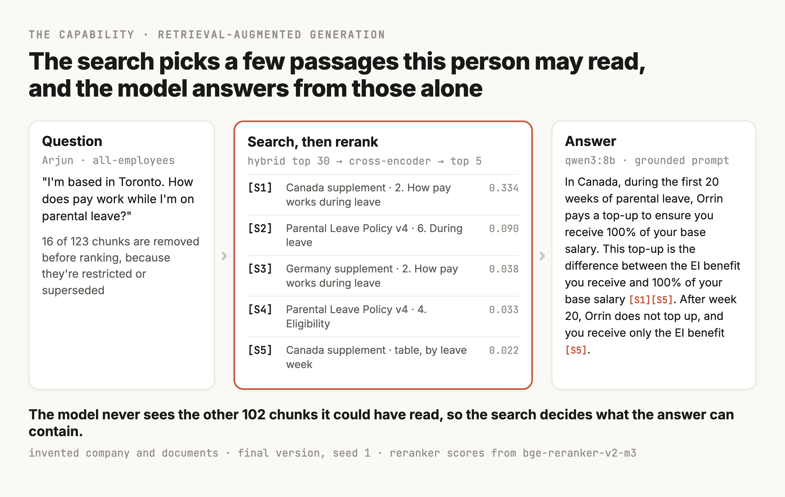
RAG can't make the model know your documents in any lasting way. Nothing is learned, so the next question starts from zero and has to be searched again. It also can't fix documents that are out of date or that contradict each other, and the model will usually repeat whichever one the search ranked first. And it can't enforce who is allowed to read what, because the model will use whatever text reaches it. Permissions have to be applied in the search, before the model sees anything, which section 5 of Part 2 builds.
Where it shows up
- An internal knowledge assistant that answers employees' questions about HR policies and engineering documents, which is the example in this module.
- A support agent that answers customers from the help center, like the flower company's agent in M6, whose
kb_passagestable is a small RAG index. - A coding agent that searches a repository and its docs before editing, like the one in M16 and M17.
- Memory lookup in M16, where the documents are facts the agent saved about past sessions.
The documents and the users change from one to the next, and all four have the same two halves, a search that has to find the right passage for this person and a model that has to answer only from what it was given.
The running example
The assistant that quoted a confidential brief to Maya
Orrin Robotics makes warehouse robots, with offices in Austin and Berlin and a controls team in Toronto. The company is made up, and so are its documents and its people. Its People Operations team and its field engineers answer the same questions every week, like how much parental leave someone gets, or what a fault code on the RC-7 controller means. So Orrin built an internal assistant that answers from 18 of its documents. Most are HR policies, with regional supplements for Canada and Germany, and engineering documents like the RC-7 fault code reference. Two are wiki pages anyone can edit, one is a scanned benefits handout, and one is a confidential brief only HR leadership can open. The documents are deliberately messy in the ways real ones are. There's an old version of the parental leave policy next to the new one, an exact copy of the time off policy exported to the shared drive, and a wiki FAQ copied from the old policy in 2024.
The first version was the one most tutorials build, and section 8 builds it. It went to a pilot group, and the six questions below came back over and over. Each one ran three times on the baseline, and the table says what came back.
| Who asks | Question | What the baseline answered |
|---|---|---|
| Maya, customer success, Austin | "How much paid parental leave do I get?" | 20 weeks in two runs. In the third it called 16 weeks "the current policy", from the old version |
| Arjun, controls engineer, Toronto | "I'm based in Toronto. How does pay work while I'm on parental leave?" | Right in all three runs, EI plus Orrin's top-up for 20 weeks |
| Lena, field service, Berlin | "The RC-7 on line 3 is showing E-1042. What does it mean and what should I do?" | Right in all three runs, an axis 2 drive overcurrent with the belt check |
| Arjun | "...How much of the leave is paid, and do I stay on the on-call rotation?" | Wrong in all three. Two runs said 16 weeks and missed the two extra weeks off the rotation. The third got the rotation right and gave no number for the pay |
| Maya | "Does the parental leave policy cover foster placements?" | "Yes, the parental leave policy covers foster placements", in all three. The policy never mentions foster placements |
| Maya | "Will people on parental leave be affected by the Q4 restructuring?" | "Employees on parental leave on 3 November 2026 are excluded from the reduction", from the confidential brief, in all three |
The last row is the one that would end the pilot. Maya can't open the leadership brief, and the assistant quoted it anyway. It did the same with the severance terms and with the security team's key rotation date, because nothing in the baseline knew who was asking.
The second and third rows passing on the baseline are worth noticing too, because later changes in this module broke questions that already worked. The context header broke the E-1042 lookup. The final version turned a correct bereavement answer into a wrong one in two of three runs, and it failed the injection test the baseline had passed. The only reason anyone noticed is that these questions were written down as test cases and rerun after every change. The eval dataset has 36 test cases in all, and section 12 describes it. Every later section starts from one of these questions going wrong, walks back to the stage where it went wrong, and measures the fix on all 36.
Do you need retrieval?
Check whether the documents fit in the prompt before you build a search
Current models accept long inputs, often hundreds of thousands of tokens, so the first question about any RAG system is whether you need the search at all. If every document fits in the request, you could send all of it with every question and let the model find the answer. Anthropic's own guidance says that "If your knowledge base is smaller than 200,000 tokens (about 500 pages of material), you can just include the entire knowledge base in the prompt" (Anthropic, September 2024).
Orrin's index is small enough to try it. The current documents Maya may read come to 107 chunks and about 41,800 characters, which is roughly 10,000 tokens at about four characters per token. So the run tried a fourth configuration, longctx, which skips the search and sends every chunk the person asking may read, in document order, with the same grounded prompt the final version uses.
On the same 35 graded test cases, three runs each, the long-context version passed 96 of 105 answers and the final RAG version passed 97, which on this many test cases is no difference at all. The failures were different, though. Long context passed the injection test in all three runs, where the final version failed all three, and a likely reason is that the planted note in the wiki was one of 107 chunks sitting next to the full policy, where the final version's search put it first of five. Long context failed Maya's restructuring question in all three runs by inventing a reassurance, "The restructuring does not impact employees on leave, and their roles and benefits remain protected as per the Parental Leave Policy", with a citation to the policy's section on what happens during leave. The final version said it couldn't find anything in all three. On time, the long-context runs took 525 seconds for 105 answers against 605 for the final version, because Orrin's documents are small and the reranker runs on a laptop CPU. On a corpus a hundred times bigger, about a million tokens, the prompt wouldn't fit in this model's context window at all.
The published comparisons point both ways. A 2024 study from Google DeepMind and the University of Michigan found that "On average, LC surpasses RAG by 7.6% for Gemini-1.5-Pro, 13.1% for GPT-4O, and 3.6% for GPT-3.5-Turbo", and that "for 63% queries, the model predictions are exactly identical" between the two (Li et al., 2024). A 2025 benchmark found the opposite at larger sizes. At 32k tokens of context, long context averaged 2.4% higher accuracy, and at 128k "this trend reversed, with RAG outperforming LC by 3.68%" (Li et al., LaRA, 2025). Longer inputs also cost accuracy on their own. Chroma tested 18 models in 2025 and found that "Even a single distractor reduces performance relative to the baseline" (Chroma, July 2025), and the 2023 "Lost in the Middle" paper found models used information best "at the beginning or end of the input context" (Liu et al., TACL 2023). Those were 2023 models and newer ones may do better, but the distractor result is from 2025.
Whichever way the accuracy comparison goes on your data, the long context still has to be the text this person may read, so you still need the permission filter from section 5 of Part 2, run before the prompt is built. It also costs more on every question, because every question sends every token. On Orrin that's about 10,000 tokens of documents per question against about 1,750 for the final version's five sources, and a real company's documents usually run to far more than Orrin's 18 files. Citations still work with the whole corpus in the prompt, and the model has more wrong sources to choose from when it cites one.
Fine-tuning a model on the documents is the other alternative people reach for, and it can't do three things this job needs. Training puts the documents into the model's weights, where you can't see which document an answer came from, can't remove a superseded policy without training again, and can't stop someone from getting an answer from a document they aren't allowed to read. Fine-tuning helps with how a model answers, like its format or its tone, which M21 covers, and it can sit on top of retrieval.
So the order is to try the whole corpus in the prompt when it fits, measure it with the same eval dataset you'd use for RAG, and build the search when the corpus doesn't fit, when the cost per question adds up, or when permissions differ between people, which at a company is almost always.
Architecture
One pipeline builds the index, and another answers the question
A RAG system is two programs that run at different times. The ingestion pipeline runs whenever a document changes. It pulls the file from wherever it lives, turns it into clean text, cuts it into chunks, attaches metadata to each chunk and writes the chunks into an index. The serving pipeline runs on every question. It works out who is asking, searches the index for chunks that person may read, picks the best few, puts them in the prompt and returns the answer with its citations.
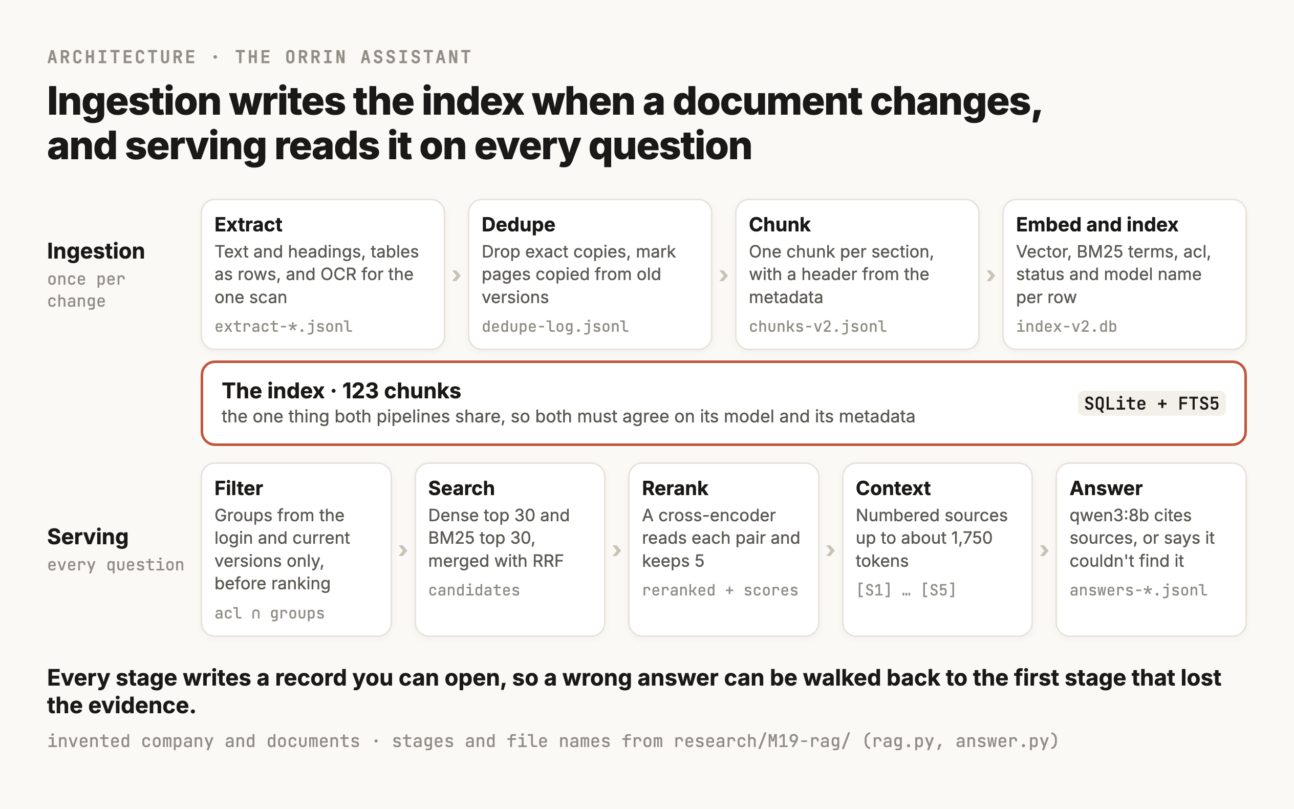
The two pipelines share one thing, which is the index, and most bugs in a RAG system come from the two sides disagreeing about it. Say ingestion embeds chunks with one model and serving embeds the question with another, or ingestion writes a chunk without the region it applies to and serving tries to filter on region. Neither side raises an error when that happens. Serving just returns worse chunks, so the answer gets worse, and nothing tells you why.
That's why every stage in this module writes down what it produced, in a file you can open and read.
| Stage | Record | What you check in it |
|---|---|---|
| Ingestion, once per document change | ||
| Extract | extract-*.jsonl, the text and sections each file produced | Is the text all there, in reading order, with tables still readable? |
| Dedupe | dedupe-log.jsonl, which files were dropped or marked and why | Did a copy of an old policy survive? |
| Chunk | chunks-*.jsonl, one row per chunk with its id, text and metadata | Does each chunk make sense alone, and does it say where it came from? |
| Index | a row per chunk in SQLite, with the embedding and the model that made it | Was every chunk embedded by the model serving uses? |
| Serving, once per question | ||
| Candidates | the dense and BM25 lists, before and after fusion | Is the right chunk anywhere in the top 30? |
| Reranked evidence | the top 5 with reranker scores | Is it in the top 5, and what outranks it? |
| Context | the numbered sources exactly as the model saw them | Did the right chunk survive the budget, and is anything here the user may not read? |
| Answer | the text with [S1] style citations mapped back to chunk ids | Does every claim cite a source that supports it? |
| Eval record | the test case, the retrieved ids, the answer and each check's result | Which check failed, and on which run? |
M2 made the same argument for agents, where a trace records every model call and tool call in one run. A RAG trace is the serving half of the table above, and the ingestion records are what let you answer the question a trace can't, which is why the right chunk was never in the index in the first place.
Embeddings
Turn every chunk and every question into a vector with one embedding model
As you already know from M3, a language model reads text as tokens, and inside the model every token becomes a long list of numbers. An embedding model is a model built to stop there. It reads a whole piece of text, a question or a chunk of a document, and outputs one list of numbers of a fixed length, called a vector or an embedding. Orrin's embedding model, BAAI/bge-small-en-v1.5, outputs 384 numbers for any text it's given, whether that's a six-word question or a 1,200-character policy section (bge-small-en-v1.5 model card).
The model is trained so that the vector for a question and the vector for a passage that answers it point in nearly the same direction, and the vector for an unrelated passage points somewhere else. Dense passage retrieval, one of the first systems to do this for question answering, trained two BERT encoders on pairs of questions and the passages that answer them, pushing each question's vector toward its passage and away from the others in the same batch (Karpukhin et al., 2020). Current embedding models are trained the same basic way, on far more pairs.
This is what bge-small produced for Arjun's question and for the chunk that answers it, the Canada supplement's section on pay. Both come from embeddings_demo.py, which prints every intermediate value used in sections 5, 6 and 11.
| The question | The chunk HR-014-CA-v2#s1.0 | |
|---|---|---|
| Text that went in | Represent this sentence for searching relevant passages: I'm based in Toronto. How does pay work while I'm on parental leave? | The context header from section 10, then "Employees in Canada apply to the federal Employment Insurance (EI) program..." |
| Tokens | 29 | 180 |
| Numbers out | 384 | 384 |
| The first eight | 0.0002, 0.0171, −0.0155, −0.0219, 0.0412, −0.0237, 0.0609, −0.0204 | −0.0794, 0.0217, −0.0304, −0.0206, 0.0325, 0.0189, 0.0794, −0.0389 |
| Length of the vector | 1.0 | 1.0 |
No single number means anything you could name. There's no dimension for "Canada" or for "pay", and the meaning is spread across all 384 numbers, so a vector on its own tells you nothing. The only useful thing to do with it is compare it with another vector from the same model, which section 6 covers. Here the two vectors scored a cosine similarity of 0.786, the highest of Orrin's 123 chunks for this question.
What the numbers capture, and what they blur
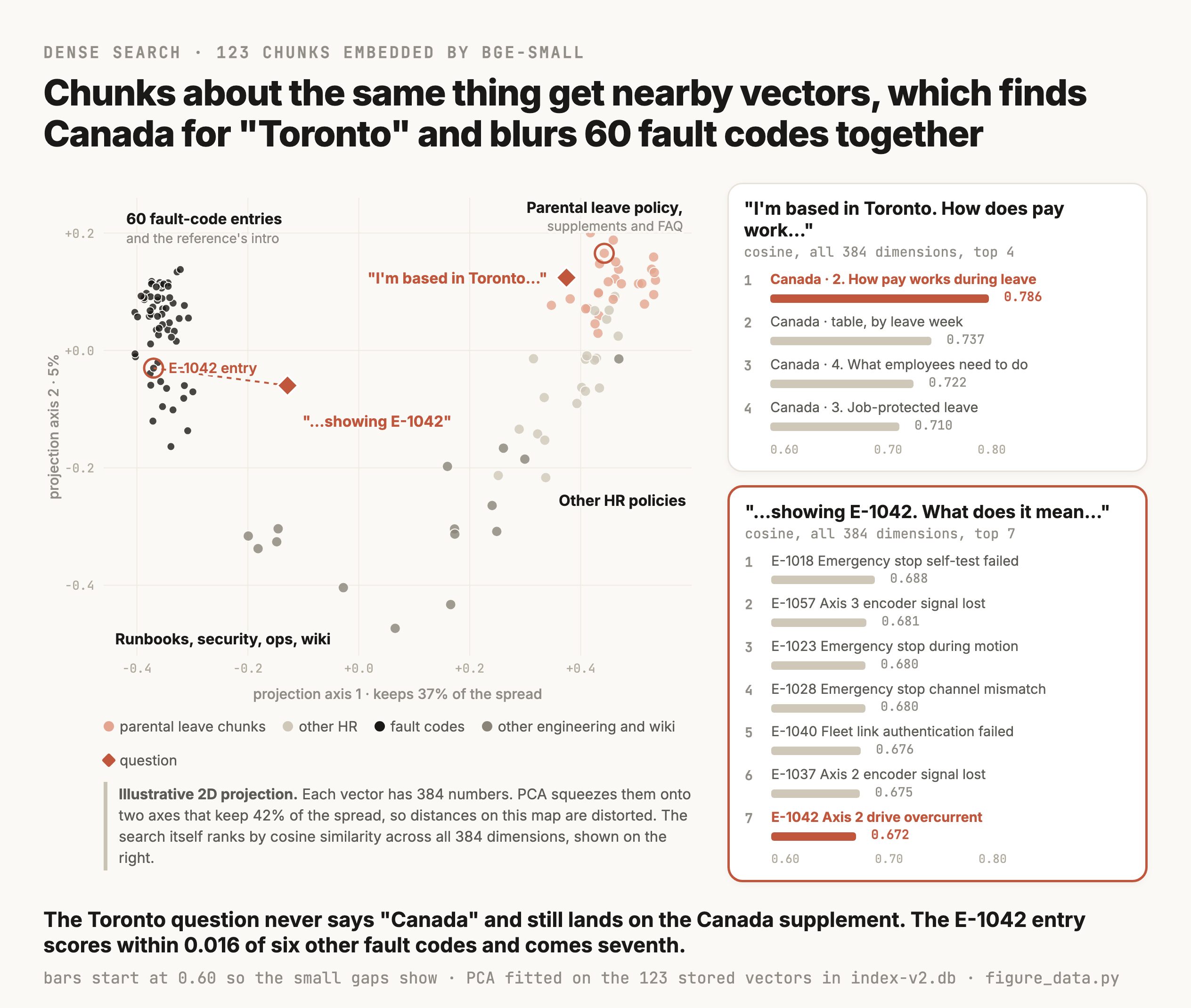
Embeddings capture what a text is about, and they do it across different wording. When the run asked "The robot's second joint motor is drawing too much current. What's wrong?", which shares no key word with the fault reference, dense search put the E-1042 entry, "Axis 2 drive overcurrent", first. Section 6 has more pairs like that one.
What they blur are the details that make one passage right and its close neighbour wrong. For Lena's E-1042 question, the E-1042 entry scored 0.672 and the E-1017 entry, an axis 2 encoder fault, scored 0.671. Both are about axis 2 on the same robot, and the vectors can't say that the code is what decides the answer. The same goes for version numbers and dates. The old parental leave FAQ, which says 16 weeks, scored higher for "How much paid parental leave do I get?" than the current policy that says 20. Section 12 treats both of these as failure types to test for.
The embedding model isn't the model that writes the answer
A RAG system has at least two models, and they do different jobs. The embedding model turns text into vectors, and it's usually small. bge-small has about 33 million parameters and embeds a question in about 15 milliseconds on the laptop's CPU. The model that writes the answer, qwen3:8b in Orrin's run, has about 8 billion parameters and never sees a vector. It gets the text of the chunks the search picked.
Because they're separate, you choose and change them separately. You can swap the answering model tomorrow and the index doesn't change at all. Changing the embedding model is different, because every stored vector came from it, so every chunk has to be embedded again. For Orrin's 123 chunks that takes seconds. For the 57,638 FiQA passages in section 7 it took 18 minutes on the laptop's CPU, and a company's whole document store takes much longer.
Questions and chunks must go through compatible encoders
The question's vector and the chunks' vectors have to come from the same model, at the same version, with the same settings, because each model places text in its own space and a distance between vectors from two models means nothing. Google's embedding docs say of their own two models that the embedding spaces "are incompatible", and that after upgrading "you must re-embed all of your existing data" (Gemini API docs, updated 17 September 2026).
A mismatch doesn't raise an error when the two models output the same number of dimensions. The run embedded Orrin's 29 questions with a different 384-number model, all-MiniLM-L6-v2, and searched the bge-small index with them. Nothing failed, and the evidence reached the top 5 for 21 of 29 questions against 27 with the right model. That's worse than it looks, because 21 looks like a working system. The two models' vectors happen to line up partly, with a cosine of 0.30 on average between their vectors for the same question, and with the other model's dimensions shuffled or with random vectors the count dropped to 2 and 0. So a deploy that points the query side at the wrong model can quietly lose a fifth of its answers. The Orrin index stores the model's name on every row, and serving refuses to query an index built by another model.
assert {r[5] for r in rows} == {EMBED_MODEL}, "index built with another embedding model"Some models also want the question and the passage marked differently. bge puts Represent this sentence for searching relevant passages: in front of queries and nothing in front of passages, which is QUERY_PREFIX in rag.py. E5 models expect query: and passage: , and their card says that without them "you will see a performance degradation" (intfloat/e5-large-v2). On Orrin's questions, dropping bge's prefix changed nothing, 27 of 29 either way, which matches its card, where the v1.5 release says "we improve its retrieval ability when not using instruction". Other models aren't so forgiving, and a missing prefix won't raise an error either, so read the card for the model you pick and test with and without. Some APIs also take a dimensions setting that returns shorter vectors, and OpenAI's docs say you can "shorten embeddings (i.e. remove some numbers from the end of the sequence)" that way (OpenAI embeddings guide). A change to that setting counts as a new model too.
Choosing an embedding model, and what domain terms do to it
The public leaderboard people check first is MTEB, which scores embedding models on dozens of tasks. Its own maintainers warned in 2025 that "The highest ranking models achieve their scores by training on benchmark tasks, even though models with lower scores might generalize better to out-of-distribution environments" (Chung et al., 2025). So the leaderboard gives you a shortlist, and your own eval dataset makes the choice. The things worth checking for each candidate are the languages your documents use, how long an input it accepts, how many numbers it outputs, since storage grows with that, and whether sending your documents to a hosted API is allowed.
On Orrin's eval, the 568-million-parameter bge-m3 put the first piece of evidence in the top 5 for 28 of 29 questions, against 27 for bge-small, a model 17 times smaller. For most questions the small model was already enough, and the one class of question both models handled badly was looking up a code, which section 12 measures on all 60 fault codes.
Domain terms are the usual reason a general embedding model gets a question wrong. Fault codes and acronyms like EI either appear rarely in the text the model was trained on or not at all, so the model has little to go on beyond the surrounding words. The fixes differ a lot in cost. The cheapest is to run keyword search next to dense search, which section 11 does. The next is to put the terms into the text that gets embedded, like the context header in section 10. The most expensive is to fine-tune the embedding model on pairs of your own questions and passages, which M21 covers.
Text past the model's limit is cut off without a warning
Every embedding model has a maximum input length, and anything longer is cut off. bge-small's is 512 tokens. OpenAI's text-embedding-3 models take 8,192 (OpenAI embeddings guide). The run embedded the whole RC-7 fault reference, 3,702 tokens, as one text, and then embedded only its first 512 tokens. The two vectors were identical, with a cosine of 1.000000, and sentence-transformers gave no warning. The cut landed in the middle of the E-1008 entry, so the other 52 entries had no effect on the vector at all, so a one-chunk-per-document index could never have found E-1058 by what its entry says.
That's the reason chunk size is measured in the embedding model's tokens, and the reason to check the longest chunk before building an index. Orrin's longest chunk in the final index is 212 tokens, well under the limit.
Semantic similarity
Compare vectors by their direction, and read the score as a ranking
Once every chunk and the question are vectors, semantic search is a comparison. The question's vector gets compared with every chunk's vector, and the chunks whose vectors are most similar come back. Vectors can be compared in a few ways, and the differences are easiest to see on vectors with just two numbers.
Three measures on three small vectors
Take a = (3, 4), b = (6, 8) and c = (4, 3). The vector b points in exactly the same direction as a and is twice as long, and c points in a slightly different direction and has the same length as a.
The dot product multiplies the numbers pairwise and adds them up. a · b is 3×6 + 4×8 = 50, and a · c is 3×4 + 4×3 = 24. It grows with length as well as with direction, so b wins partly because it's long.
Cosine similarity divides the dot product by both lengths, which leaves only the angle between them. The length of a is √(3² + 4²) = 5, the length of b is 10 and the length of c is 5. So cosine for a and b is 50 / (5 × 10) = 1.0, the most similar two vectors can be, and for a and c it's 24 / (5 × 5) = 0.96. Cosine runs from −1 to 1, and it ignores length completely.
Euclidean distance, also called L2 distance, is the straight-line distance between the two points, and smaller means more similar. From a to b it's √(3² + 4²) = 5, and from a to c it's √(1² + 1²) = 1.41. So by distance c is the closer one, while cosine says b is.
The three measures disagree here because the vectors have different lengths. Normalizing a vector means dividing it by its length so the length becomes 1. a becomes (0.6, 0.8), and so does b, since it pointed the same way, and c becomes (0.8, 0.6). After that, the dot product equals the cosine, and the distance from a to b is 0 and from a to c is 0.28, so all three measures rank b first. For vectors of length 1 this always holds, because the squared distance is 2 − 2 × cosine, which you can check with 0.28² ≈ 2 − 2 × 0.96.
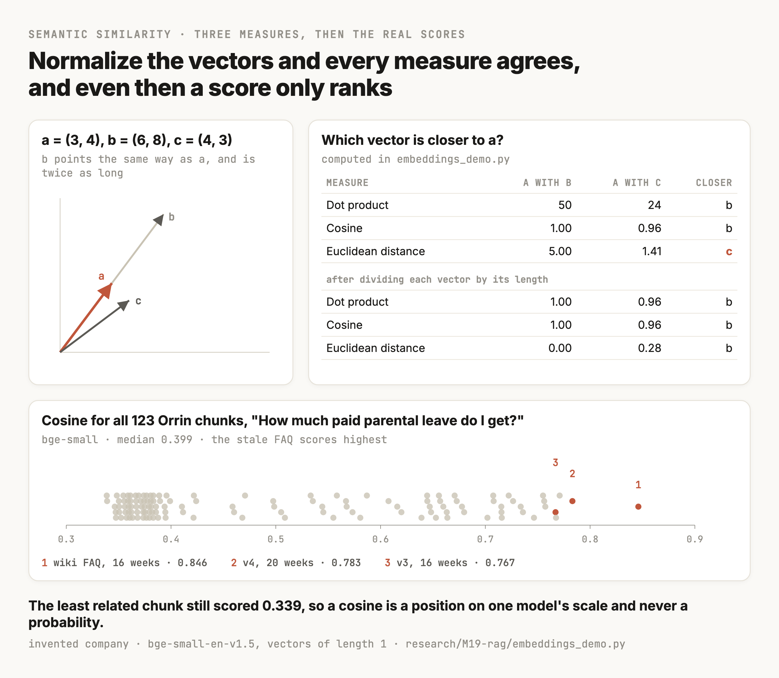
bge-small ends with a normalization step, so every vector it outputs already has length 1. The run checked all 123 chunk vectors, and their lengths were all 1.0. That's why mat @ q in rag.py, a plain dot product, is cosine similarity. OpenAI's docs say the same about their embeddings, that they "are normalized to length 1", so "Cosine similarity and Euclidean distance will result in the identical rankings" (OpenAI embeddings guide). Vector databases name the measure explicitly. pgvector has <=> for cosine distance, <-> for L2 distance and <#> for the negative inner product, and its README says "If vectors are normalized to length 1 (like OpenAI embeddings), use inner product for best performance" (pgvector). Chroma's default is "l2 (squared L2 norm)" (Chroma docs), which ranks the same as cosine only when the vectors are normalized. If you store unnormalized vectors and pick the dot product, long chunks can win because they're long, so check what the model outputs and what the index measures.
How semantic search matches different wording
Semantic search finds a passage that says the same thing in other words, which keyword search can't. The run asked five questions worded differently from the passage that answers them and recorded where each search put that passage among Orrin's 123 chunks.
| Question | The passage | Cosine | Dense rank | BM25 rank |
|---|---|---|---|---|
| "How much time off do I get after having a baby?" | HR-014 v4, "Every eligible parent receives 20 weeks..." | 0.732 | 2 | 19 |
| "My dad passed away. How many days can I take?" | HR-023, "up to 10 working days... death of a spouse, partner, child or parent" | 0.624 | 1 | 6 |
| "Can I work from Spain for a few weeks without asking anyone?" | HR-030, "more than 14 days in a calendar year" | 0.579 | 2 | 4 |
| "What extra pay do engineers in Berlin get for being on call?" | ENG-OPS-005, "400 USD, 500 CAD or 350 EUR per rotation week" | 0.720 | 1 | 1 |
| "The robot's second joint motor is drawing too much current. What's wrong?" | E-1042, "Axis 2 drive overcurrent" | 0.719 | 1 | 5 |
Dense search put the answer first or second every time. BM25 put the baby question's answer 19th, because the entitlement section never says "baby" or "time off", and the only words it shares with the question are common ones. The one question BM25 got right, the Berlin one, shares the word "engineers" with its passage. When the baby question's answer came second on dense search, the chunk ahead of it was a section of the old wiki FAQ, which is the next problem.
The map below squeezes Orrin's 384-number vectors onto two axes so you can see the groups the model forms.
Similar isn't the same as relevant
A high similarity says the passage is about what the question is about. It doesn't say the passage answers the question, and the gap between those two is where most dense-search mistakes come from.
| Question | Passage | Cosine | Answers it? |
|---|---|---|---|
| "How much paid parental leave do I get?" | Wiki FAQ copied from version 3, "16 weeks" | 0.846 | No, out of date |
| HR-014 v4 entitlement, "20 weeks" | 0.783 | Yes | |
| HR-014 v3 entitlement, "16 weeks" | 0.767 | No, superseded | |
| "I'm based in Toronto. How does pay work while I'm on parental leave?" | Canada supplement, how pay works | 0.786 | Yes |
| Germany supplement, how pay works | 0.708 | No, wrong country | |
| "The RC-7 on line 3 is showing E-1042..." | E-1042, axis 2 drive overcurrent | 0.672 | Yes |
| E-1017, axis 2 encoder count mismatch | 0.671 | No, wrong fault |
The stale FAQ scored highest of all, because its question heading, "How much leave do I get?", is almost the user's question. The Germany section is about exactly the same thing as the Canada one, for a different country. And two fault entries about axis 2 differ by 0.001. In each pair, the passage that answers differs from its neighbour in one small detail, and the vector barely registers it. The fixes are elsewhere in the pipeline, with metadata filters for version and region (section 6 of Part 2), keyword search for codes (section 11) and a reranker that reads the question and the passage together (section 11).
A score isn't a probability, so thresholds need your own data
A cosine of 0.786 doesn't mean a 79% chance the passage is relevant. It's a position on a scale that depends on the model, and bge's scale is compressed. For "How much paid parental leave do I get?", every one of Orrin's 123 chunks scored between 0.339 and 0.846, with a median of 0.399, so the least related chunk of all, the E-1025 entry about a safety network fault, still scored 0.339 for a question about parental leave. bge's model card says "the similarity distribution of the current BGE model is about in the interval [0.6, 1]", and that "what matters is the relative order of the scores, not the absolute value", and it tells you to "select an appropriate similarity threshold based on the similarity distribution on your data" (bge-small-en-v1.5 model card).
So could a threshold on the top score tell the assistant when the documents don't have the answer? The run recorded the best cosine for every test case, after the permission filter.
| Kind of test case | Test cases | Lowest best score | Highest best score |
|---|---|---|---|
| Answerable, including multi-document and the injection test | 28 | 0.596 (e1042-returns) | 0.870 |
| Nothing in the documents answers it | 4 | 0.614 (sabbatical) | 0.747 (foster) |
| The asker may not read the answer | 3 | 0.593 (severance) | 0.728 (reorg) |
The ranges overlap almost completely. foster, which should be refused, scored higher than 11 answerable questions, so any threshold that refused it would also refuse those 11. The reranker's scores in section 11 separate the two groups much better, and even that threshold was picked on the same test cases it was judged on. A threshold picked on one model's scores also doesn't carry over to another model, since each has its own scale. If you want one, pick it from a labeled sample of your own questions, measure how many answerable ones it refuses, and pick it again whenever the model changes.
Vector databases
Put the vectors in an index built for nearest-neighbour search
Dense search, the way section 6 described it, is one line of numpy. Every chunk's vector sits in a matrix, the question's vector gets multiplied against all of them, and the five highest scores win. That's called exact search, because it compares the question with every chunk and so always finds the true closest ones, and on Orrin's 123 chunks it's fast enough that nothing else is needed. A real company has millions of chunks, though, and comparing the question with every one of them on every request gets slow. A vector database solves that. It stores each chunk's vector next to its id and metadata, and it keeps an index that finds the closest vectors while only comparing the question with a small fraction of them. That's where semantic search usually runs in a production RAG system, and it's why "RAG" and "vector database" get used as if they were one thing.
They aren't quite one thing. Semantic search needs embeddings and a way to find the nearest ones, and a vector database is the usual way, while plain keyword search with BM25 needs neither, and small corpora can use exact search like Orrin's. What the vector database adds is speed at scale, plus the things you'd expect of any database, like keeping the data safely on disk and filtering on metadata.
What a row holds
| Field | Example | Why it's there |
|---|---|---|
| Id | HR-014-CA-v2#s1.0 | Citations and eval records point at it |
| Vector | 384 numbers from bge-small | What the nearest-neighbour search compares |
| Text | The chunk with its context header | What goes into the prompt, and what BM25 indexes |
| Metadata | acl, status, version, region, source | What the filters in sections 5 and 6 of Part 2 run on |
| Embedding model | BAAI/bge-small-en-v1.5 | So serving refuses to compare vectors from two models |
You can also keep only the id and the vector in the vector database and look up the text and metadata in your main database afterwards. That works, and it means the filter can't run inside the vector search, which is the problem the filtering subsection below measures.
How an approximate index finds neighbours without checking every row
The index most of them use, including pgvector's and Chroma's, is HNSW, short for Hierarchical Navigable Small World graphs (Malkov and Yashunin, 2018). When a vector is added, the index links it to a handful of its nearest neighbours, so the whole collection becomes a graph where each point knows who's near it. A few points are also copied into sparser layers on top, with longer links, so a search can cross the whole collection in a few long jumps before it starts looking closely. A search starts at the top layer, walks greedily toward the question's vector, drops down a layer, and keeps walking until it reaches the bottom layer, where it keeps a list of the best candidates found so far and returns the top k.
You control the trade with three settings, where m is how many links each point keeps, ef_construction is how hard the index looks for good neighbours while building, and ef_search is how many candidates the search keeps while walking. A bigger ef_search checks more of the graph, so it finds more of the true neighbours and takes longer. pgvector's defaults are an m of 16, an ef_construction of 64 and an ef_search of 40, and its README says approximate indexes "trade some recall for speed", where exact search "provides perfect recall" (pgvector). Recall here means agreement with exact search, the share of the true five nearest vectors the index returns, which M6 introduced. It says nothing on its own about whether those vectors hold the answer.
What the index did with Orrin inside a bigger corpus
To see the trade on something bigger than Orrin, the run put Orrin's 123 chunks into one index with the 57,638 passages of FiQA, a public dataset of financial questions and answers from the BEIR benchmark, and embedded them all with the same bge-small model, 57,761 vectors in all. Then it ran Orrin's 29 questions with known evidence and 300 of FiQA's test questions through exact search, through an HNSW index built with hnswlib at pgvector's default m and ef_construction, and through Chroma, an open-source vector database that runs inside a Python process, with its default settings and cosine distance.
| Search | Median time per question | Agreement with exact top 5, all questions | Orrin questions | FiQA questions | Orrin questions with evidence in top 5 |
|---|---|---|---|---|---|
| Exact, numpy over every row | 4.2 ms | 100% | 100% | 100% | 21 of 29 |
HNSW, ef_search 10 | 0.08 ms | 75.8% | 50.3% | 78.3% | 9 of 29 |
HNSW, ef_search 40, pgvector's default | 0.18 ms | 91.4% | 77.9% | 92.7% | 14 of 29 |
HNSW, ef_search 100 | 0.37 ms | 96.4% | 89.0% | 97.1% | 19 of 29 |
HNSW, ef_search 200 | 0.63 ms | 98.1% | 94.5% | 98.5% | 20 of 29 |
Chroma 1.5.9, defaults (ef_search 100) | 0.86 ms | 97.8% | 98.6% | 97.7% | not measured |
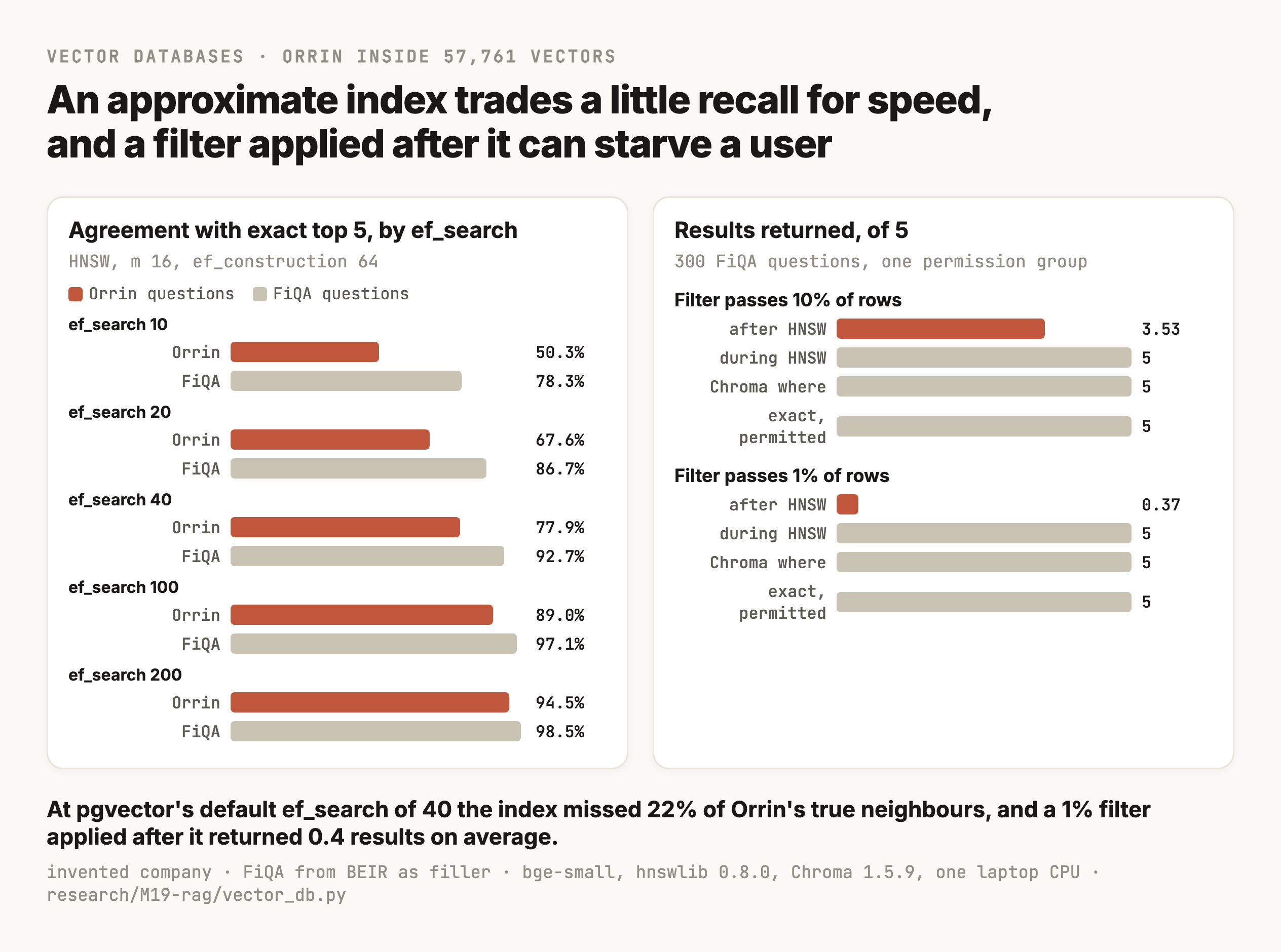
The index was 23 times faster than exact search at pgvector's default setting, and it found 91% of the true neighbours overall, which sounds like a fine trade until you split it by question. On FiQA's questions it agreed with exact search 93% of the time, and on Orrin's it agreed 78% of the time, so the evidence for Orrin's questions reached the top 5 for 14 questions where exact search managed 21. The likely reason is that Orrin's 123 chunks are a small, tight cluster in a graph built mostly from finance posts, and a greedy walk that only keeps 40 candidates misses some of the cluster's members. Raising ef_search to 200 got most of that back for under half a millisecond more. Chroma's defaults, which build and search with 100 candidates, matched exact search on 98.6% of Orrin's slots. None of this showed in the average, which is why you measure recall on your own questions and on each kind of document you care about, the same point M6 made for pgvector.
With FiQA in the same index, exact search itself found Orrin's evidence for only 21 of 29 questions, against 27 on Orrin's 123 chunks alone, because 59 of the 145 slots in Orrin's top-5 lists went to finance posts. That comes from putting unrelated documents in one index with no filter, and the fix is the filter in the next subsection.
Building the HNSW index over 57,761 vectors took 18 seconds, and the saved index file was 93 MB against 85 MB for the raw vectors. Embedding the 57,638 FiQA passages took 18 minutes on the laptop's CPU, which is the ingestion cost to remember when someone proposes changing the embedding model, since every row has to be embedded again and the index rebuilt.
Filter before ranking, never after
Every search in the final version applies two filters, the user's groups and the document's status, and it applies them before ranking. In the Orrin run that's a mask checked on every chunk before it can be a candidate, and in SQL it's a WHERE clause in the same query that ranks.
The order makes a difference with an approximate index. The pgvector README says that "With approximate indexes, filtering is applied after the index is scanned. If a condition matches 10% of rows, with HNSW and the default hnsw.ef_search of 40, only 4 rows will match on average" (pgvector). Elastic's docs say the same about their engine, that post-filtering "can return fewer than k results, even when enough relevant documents exist" (Elastic). The run measured it on the 57,761-vector index, where every FiQA passage got a random permission group, so one group's filter lets through either 10% or 1% of rows, and 300 FiQA questions were each asked by a user in one group.
| How the filter runs | Filter passes 10%, results returned | Agreement with exact | Filter passes 1%, results returned | Agreement with exact | Median time at 1% |
|---|---|---|---|---|---|
| After HNSW's 40 candidates, like pgvector by default | 3.5 of 5 | 66% | 0.4 of 5 | 7% | 0.25 ms |
| During the HNSW search, hnswlib's filter callback | 5 of 5 | 98% | 5 of 5 | 99.8% | 7.7 ms |
Chroma's where filter | 5 of 5 | 99.6% | 5 of 5 | 100% | 23 ms |
| Exact search over only the permitted rows | 5 of 5 | 100% | 5 of 5 | 100% | 0.2 ms |
Filtering after the search returned 3.5 results on average at 10%, close to the README's 4, and at 1% it returned fewer than one, so every one of the 300 users got a short or empty list with nothing in any log to say why. Filtering during the search always returned five, and it got slower as the filter got stricter, because the walk has to pass more rejected points before it finds five it may return. Chroma returned the exact answer at both filter levels, and its docs don't say how its filter is applied, so the only thing to go on is this measurement. For the 1% filter, plain exact search over the 560 permitted rows was the fastest and the most accurate of all, as long as the database can find those rows quickly, which in Postgres means an ordinary index on the group column. That's the pgvector README's advice for selective filters too.
Which way is right depends on how many rows the filter lets through. When it lets through a small share of rows, like one customer's documents in a product with many customers, search only those rows exactly, or keep them in their own partition or table, which pgvector recommends for tenants as "list partitioning or separate tables". When it lets through most rows, like "current documents only", let the engine filter during the search. pgvector 0.8.0 added iterative index scans for that, which keep scanning until enough rows pass the filter or hnsw.max_scan_tuples, 20,000 by default, is reached, and the current release is 0.8.6. Qdrant builds extra links into its graph for indexed metadata fields and switches to a full scan when a filter is selective enough, and its docs warn that "the HNSW graph starts to fall apart when using filters that are too strict" (Qdrant). Whatever the engine, test it with your most restrictive user, since that's where filtered search loses results.
The figure puts the recall split and the filtering results next to each other.
Keeping the index up to date, and what it costs in memory
A vector index keeps changing after it's built, because documents change every day, so it has to take new and changed rows and drop deleted ones, and HNSW handles those less gracefully than an ordinary database index. Adding a row means linking it into the graph, which costs a search for every insert, and pgvector's README notes that "it's faster to create an index after loading your initial data". Deleting a row usually marks it as deleted and leaves its links in the graph until a cleanup, which in Postgres is a vacuum, and the README says "Vacuuming can take a while for HNSW indexes. Speed it up by reindexing first" (pgvector). In practice the sync from section 6 of Part 2 deletes and re-adds by chunk id whenever a document changes, which is why the ids have to stay stable, and a rebuild gets scheduled once enough rows have changed.
Memory is the other cost. A vector of 384 numbers stored as 4-byte floats takes 1,536 bytes, so a million chunks is about 1.5 GB of raw vectors before the graph's links, and a model with 3,072 dimensions makes that about 12 GB. In the run, the HNSW index file for 57,761 vectors was 93 MB against 85 MB for the raw vectors. HNSW is fastest when the whole graph sits in memory, and pgvector's README says "Indexes build significantly faster when the graph fits into maintenance_work_mem". The dimensions setting from section 5 and half-precision storage, which pgvector supports, are the usual ways to cut it.
Choosing where the vectors live
Vector search is sold in a few shapes, and what separates them is how much of a database you get around the index.
| Kind | Examples | What you get | Fits when |
|---|---|---|---|
| An extension to a database you already run | pgvector for Postgres | Vectors in the same tables and transactions as the rest of your data, with SQL filters and row-level security | You already run Postgres, and recall and latency measured on your own queries are good enough |
| A dedicated vector database | Qdrant, Pinecone, Weaviate, Milvus, Chroma | Indexing, metadata filtering, updates and scaling built around vectors | Vector search load would slow your main database, or you need features it lacks |
| A search engine with vector fields | Elasticsearch, OpenSearch | BM25, vectors and filters in one engine, so hybrid search is one query | You already run one for keyword search |
| A library | FAISS, hnswlib | The index alone, with no storage of rows and no filters or access control | You build the database parts yourself, or for experiments like this one |
Which of these fits depends on a few requirements, and they decide most choices.
| If you need | Start with | Because |
|---|---|---|
| Vectors next to permissions and other data, with transactions and row-level security | pgvector | The permission filter from section 5 of Part 2 is a WHERE clause on the same row |
| BM25 and vector search in one request | Elasticsearch or OpenSearch | Both indexes live in one engine, so hybrid search is one query |
| No servers to run | A hosted vector database such as Pinecone | The provider runs and scales the index |
| Heavy metadata filtering on your own servers | Qdrant | Its docs describe filtering inside the HNSW search, the approach that returned full lists in this section's measurements |
| A prototype, tests or a notebook | Chroma, FAISS or hnswlib | They run inside your process with no server |
Features in this space change every few months, so treat the table as where to start reading, and decide on measured recall and latency for your own queries and your own most restricted user.
FAISS's own paper describes it as "dedicated to vector similarity search, a core functionality of vector databases" (Douze et al., 2024), which is the split in the last row. For Orrin, where Postgres already holds the passages from M6, pgvector is the natural home, and the same acl and status columns carry the filters from sections 5 and 6 of Part 2. The choice between the others is the one M6 described, which is to move when measured recall or latency on your own queries says the current one can't keep up, since every extra system is another copy of the knowledge base to keep in sync.
An index built for one embedding model is useless for another, so a model change means a new index built next to the old one and a switch in one deploy, which M6 walks through.
The baseline
Build the simplest version first, and keep it as the baseline
Before any of the techniques later in this module, build the version most tutorials build, run it on real questions and keep it. You need it for two reasons. It tells you whether the problem needs anything more, and every later change gets measured against it, so you can say what each one bought you.
The Orrin baseline, like every version in this module, runs on a laptop. The code is in research/M19-rag/ and it's simplified on purpose, with no connectors or retries, and no auth beyond a list of groups per user. It's there to show the mechanism and to produce numbers you can reproduce, so don't take it as a production design.
| Part | What the run uses | What a production system would usually use |
|---|---|---|
| Language | Python 3.11 | The same, or your service's language |
| Index | SQLite 3.41, with FTS5 for BM25 and embeddings stored as blobs | Postgres with pgvector (M6), a vector database like Qdrant or Pinecone, or a search engine like OpenSearch (section 7) |
| Vector search | Exact cosine similarity with numpy over 123 chunks | An approximate index such as HNSW once exact search gets slow (section 7) |
| Embeddings | BAAI/bge-small-en-v1.5 through sentence-transformers 6.1, on CPU | A hosted or self-hosted embedding model you've tested on your own questions |
| Reranker | BAAI/bge-reranker-v2-m3, a cross-encoder, on CPU | The same kind of model on a GPU, or a hosted rerank API |
| PDF text | PyMuPDF 1.27 | A layout-aware parser such as Docling |
| Generation | qwen3:8b through Ollama 0.34, thinking off, temperature 0.6 | Whichever model your eval picks |
The baseline takes whatever text each file gives and cuts it into 800-character pieces with 100 characters of overlap. Then it embeds every piece, and for each question it sends the five closest pieces to the model with a short prompt of the kind tutorials use.
def extract_naive(meta: dict, path: Path) -> Doc:
    """What a first pipeline does: take whatever text the file gives you."""
    if meta["format"] == "md":
        text = path.read_text().split("---", 2)[2]
    else:
        pdf = RAW / f"{meta['doc_id']}.pdf"
        text = "".join(page.get_text() for page in fitz.open(pdf))  # scan -> ""
    return Doc(meta["doc_id"], meta["title"], meta, text)


def chunk_fixed(doc: Doc, size: int = 800, overlap: int = 100) -> list[Chunk]:
    text, out, start, n = doc.text.strip(), [], 0, 0
    while start < len(text):
        piece = text[start:start + size]
        out.append(Chunk(f"{doc.doc_id}-v{doc.meta.get('version','')}#c{n}",
                         doc.doc_id, piece, piece, doc.meta))
        start, n = start + size - overlap, n + 1
return outdef dense(index, query: str, k: int, mask) -> list[int]:
db, ids, info, mat = index
q = embedder().encode([QUERY_PREFIX + query], normalize_embeddings=True)[0]
scores = mat @ q # exact cosine; production uses ANN
order = [i for i in np.argsort(-scores) if mask(ids[i])]
return [ids[i] for i in order[:k]]QUERY_PREFIX is bge's query instruction from section 5, and mat @ q is cosine similarity because every vector has length 1, which section 6 explains.
The prompt is the kind you'll find at the top of most RAG tutorials.
Use the following pieces of retrieved context to answer the question. If you don't know the answer, just say that you don't know. Keep the answer concise.
Context: {the five chunks, joined}
Question: {question}
To run it, install the pinned packages in requirements.txt, pull qwen3:8b with Ollama and run python build.py, then python eval_retrieval.py and python eval_answers.py baseline. The versions are pinned because they matter. An earlier run of the same code in another Python environment gave different dense rankings among the 60 near-identical fault-code chunks, with E-1042 at rank 31 there and rank 7 here, so every number in this module comes from one environment, and run_all.sh reruns all of them. The build reads the 18 source files and writes the three indexes, along with every record in the table from section 4. On the baseline it produced 50 chunks, and it reported that one file, the scanned benefits handout, gave no text at all. Nothing downstream complained about that, and section 9 comes back to it.
Build a minimal RAG baseline in Python for the documents in corpus/. Use SQLite for storage, BAAI/bge-small-en-v1.5 from sentence-transformers for embeddings (prefix queries with "Represent this sentence for searching relevant passages: " and never prefix passages), and exact cosine search with numpy. Split each document's text into 800-character chunks with 100 characters of overlap. Store for every chunk its id, the document id, its text, the document's metadata as JSON and the name of the embedding model. Write every chunk to out/chunks-baseline.jsonl so I can read them. Answer questions from the top 5 chunks with qwen3:8b through Ollama's /api/chat. Add an assertion at query time that every stored row was embedded by the model you're querying with. Don't add reranking or filtering yet.
Parsing, tables and OCR
Extraction decides what every later stage can see
Everything after extraction works on the text extraction produced, so a document that extracted badly can't be found by any search you build on top of it. Extraction bugs are also the quietest ones, because an empty or scrambled document still gets chunked and indexed without an error.
A scanned page gives no text, and nothing complains
The 2026 benefits handout is a one-page scan, an image inside a PDF with no text layer. PyMuPDF returned zero characters for it. The baseline chunker turned zero characters into zero chunks, so the one document that lists every region's benefits side by side was never in the index, and the build finished normally. The only sign was a line in the build's output listing files with empty extractions, and nobody reads build output unless something fails.
The fix has two parts. First, make an empty extraction fail loudly. A check that flags any PDF page with fewer than, say, 50 characters of text catches scans and PDFs whose text layer is broken. Then send those pages to OCR, which reads the text off the image. The Orrin run used qwen2.5vl:3b, a small vision model, asked to transcribe the page and write the table as a Markdown table. The transcription the index uses got every cell of the table right, and it left out the title and the date line above the table, so it never said it was the 2026 handout. A timed rerun with ocr.py, at temperature 0 and with a slightly different prompt, took 10.3 seconds on the laptop, got the cells right again, and this time kept the title. So the same model on the same page doesn't always keep the same lines. The section 10 fix covers the missing title, because the chunk header comes from the document's metadata and doesn't depend on what OCR kept. One page is a spot check, though, and before you trust OCR across thousands of scans you'd compare a sample of transcriptions with the images by hand.
A PDF table comes out as one cell per line
The Canada supplement is a two-column PDF with a small table at the end. PyMuPDF put the columns in the right order on this page, which simple extractors don't always manage, but the table came out like this.
5. Summary by leave week
Leave
weeks
EI
benefit
Orrin
top-up
Total pay
1 to 20
Yes
Yes
100% of base
salary
21 onward
If eligible
No
EI benefit only
A person can work out that Yes under Orrin top-up belongs to weeks 1 to 20, but a chunk holding half of that column can't be matched to a question about top-up pay. The structured extractor finds the table with PyMuPDF's find_tables() and writes each row with its column headers, so a row still makes sense when it ends up in a chunk on its own.
def table_rows_to_text(rows: list[list[str]]) -> str:
    """Write each table row as 'header: value' pairs so a row still makes sense alone."""
    head = [re.sub(r"\s+", " ", h or "").strip() for h in rows[0]]
    lines = []
    for r in rows[1:]:
        cells = [re.sub(r"\s+", " ", c or "").strip() for c in r]
        lines.append("; ".join(f"{h}: {c}" for h, c in zip(head, cells)))
    return "\n".join(lines)
That turned the table into Leave weeks: 1 to 20; EI benefit: Yes; Orrin top-up: Yes; Total pay: 100% of base salary. The same function handles the Markdown table in the drive-fault runbook, whose E-1042 row became Fault: E-1042; Site staff may clear: Yes; Clears allowed per shift: 1; Escalate to: Field service, and that row is the evidence for "how many times can I clear E-1042 in a shift".
The same PDF had two smaller problems. Every line break from the page layout was still in the text, so "People Operations Canada" was split over two lines and the email address had a hyphen in the middle. And the page footer, "Printed copies are uncontrolled", came out as the last line of the policy text, where a chunk would carry it as if it were part of the contact section. The structured extractor joins wrapped lines back into sentences and uses the numbered headings to split the text into sections. One column break still landed in the middle of a sentence in section 3, "depends on the employment standards of their province or / territory", which is the kind of thing you only find by reading the extraction.
Use a layout-aware parser once your documents need one
Hand-written extraction was enough for 18 files. Real document sets have multi-column layouts and tables that run across pages, plus scans of every quality, and for those you'd use a parser that models page layout. Docling, from IBM, "understands detailed page layout, reading order, locates figures and recovers table structures" and "optionally applies OCR, e.g. for scanned PDFs" (Docling technical report, 2024). Its latest release was v2.130.0 on 22 September 2026, and unstructured, another open-source option, released 0.27.10 on 27 September 2026, so both are actively maintained. Hosted services from the cloud providers do the same job. Whichever you pick, run it on a sample of your own worst documents and read the output, because the parser's benchmark scores come from other people's documents.
There's also an approach that skips text extraction. ColPali embeds an image of each page with a vision-language model and searches those embeddings directly. On the ViDoRe benchmark of visually rich pages, it scored 81.3 average nDCG@5 against 65 to 67 for pipelines that extracted text with OCR or captions first, and it indexed a page in 0.39 seconds against 7.22 (Faysse et al., ICLR 2025). That's one benchmark of charts and scanned forms, and the pages it returns are images, so the model answering needs to read images and your citations point at pages. It's worth testing when much of your knowledge lives in diagrams and scanned forms.
Chunking and context
Chunk along the document's own structure, and label every chunk
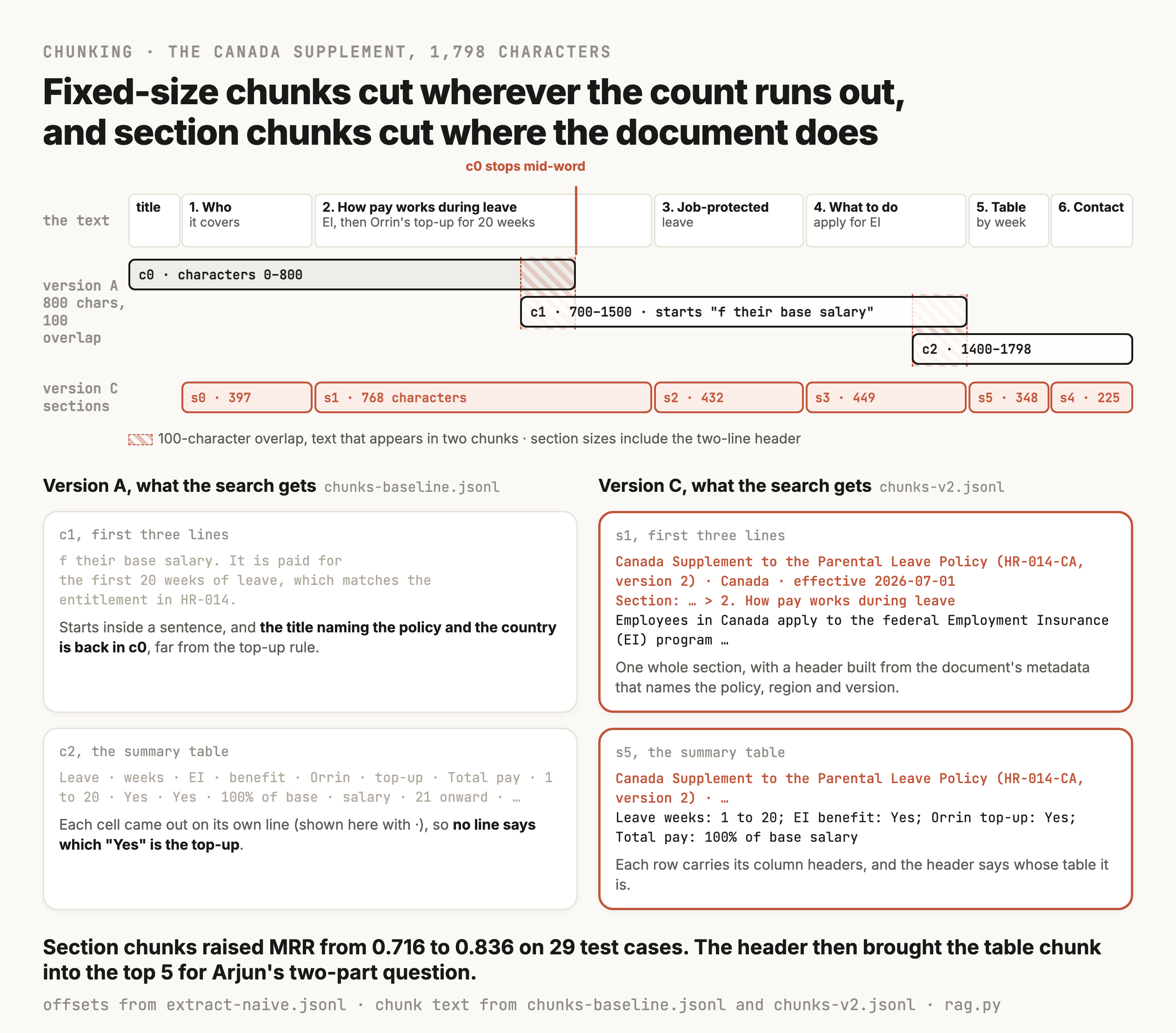
A chunk is the unit the search returns, so it has to hold an answer and make sense when it arrives with no neighbours. Fixed-size chunks break both rules in obvious ways. The baseline's second chunk of the Canada supplement starts with f their base salary. It is paid for the first 20 weeks of leave, the tail of a sentence whose start is in the previous chunk. And neither of those chunks mentions the words "parental leave" near the top-up rule, because the heading that says what the document is about sits 800 characters earlier.
Split on headings, and cap the size
The structured chunker makes one chunk per section of the document, using the headings extraction kept, and splits a section on paragraph breaks only if it's longer than 1,200 characters. On Orrin's documents that gave 123 chunks, one per policy section or fault code, against the baseline's 50.
The evidence on chunking methods says the simple choices hold up well. Chroma's 2024 study found a recursive splitter at 200 tokens with no overlap "consistently high performing", and it found OpenAI's default at the time, 800 tokens with 400 of overlap, gave "slightly below-average recall and the lowest scores across all other metrics" on its dataset (Chroma, July 2024). Vectara's study of semantic chunking, which splits wherever an embedding model thinks the topic changes, concluded its cost is "not justified by consistent performance gains" (Qu et al., 2024). The most recent study found, in August 2026, that "computationally expensive methods rarely provide consistent gains over simpler chunking", and that the best strategy depends on "the embedding model, dataset, corpus size, and target retrieval metric" (Caspari et al., CIKM 2026). All three are measured on other people's documents, and they agree on one practical point, which is that you should pick a simple splitter and measure it on your own questions before trying anything clever.
Put the document's name and section at the top of every chunk
The second fix is a context header. Before a chunk is embedded and indexed, the chunker writes the document's title, id, version, region and effective date at the top, followed by the section path.
Canada Supplement to the Parental Leave Policy (HR-014-CA, version 2) · Canada · effective 2026-07-01
Section: Canada Supplement to the Parental Leave Policy > 2. How pay works during leave
Employees in Canada apply to the federal Employment Insurance (EI) program for maternity ...
Every value in that header comes from metadata, so it costs nothing to produce. Anthropic's contextual retrieval does a more expensive version, asking a model to write 50 to 100 tokens explaining where each chunk sits in its document. On Anthropic's own tests that cut the share of questions whose evidence missed the top 20 from 5.7% to 3.7%, and to 2.9% when the same context also went into the BM25 index (Anthropic, September 2024). Anthropic priced it at $1.02 per million document tokens with prompt caching. That's a vendor's measurement on its own four datasets, and the header above gets you part of the way for free, so try the free one first.
What the chunking changes did on Orrin's questions
| Version | Chunks | Evidence in top 5 | MRR | Test cases that lost their evidence |
|---|---|---|---|---|
| A: 800 characters, no header | 50 | 27 of 29 | 0.716 | foster, e1042-returns |
| B: one chunk per section | 123 | 26 of 29 | 0.836 | multi, foster, e1017 |
| C: sections with a context header | 123 | 27 of 29 | 0.781 | e1042, e1017 |
"Evidence in top 5" counts test cases where every piece of evidence the answer needs was in the five chunks returned, and MRR, the mean reciprocal rank, averages 1 divided by the rank of the first useful chunk, so it's 1.0 when the right chunk always comes first. Section 12 works through both.
The top-5 count hardly moved, and a table like this is why you look at which test cases changed. Section chunks put the first useful chunk higher (MRR 0.716 to 0.836), because a chunk about one thing matches a question about that thing more closely than 800 characters covering three things. They also lost multi, Arjun's question about pay and the on-call rotation. The on-call half was fine, and the pay half had two places to come from, the section on how pay works and the table chunk, and neither made the top 5. The table chunk is the clearest case, because on its own it's two rows, Leave weeks: 1 to 20; EI benefit: Yes; Orrin top-up: Yes; ..., which never say "Canada" or "parental leave".
The header fixed that. With "Canada Supplement to the Parental Leave Policy" and "Canada" at the top of the table chunk, it came fourth for multi, and foster got the entitlement section back into its top 5. It also broke e1042. Every one of the 60 fault-code chunks now starts with the same line, "RC-7 Controller Fault Code Reference (ENG-RC7-FAULTS, version 7.3)", and to a small embedding model those 60 chunks became more alike than they were, so the entry for E-1042 fell from first to seventh. The next section fixes that with a search that matches the code itself, which is also why the chunks keep their header.
Metadata every chunk carries
chunk_id, stable across rebuilds, likeHR-014-CA-v2#s1.0, so logs and eval records from last month still point at something.doc_id,version,statusandeffective, so serving can drop superseded versions (section 6 of Part 2).acl, the groups allowed to read the source, copied from the source system at ingestion (section 5 of Part 2).region,ownerandsource, so answers can prefer the right supplement and so every wrong chunk has someone to fix it.- The hash of the text and the name of the embedding model, so the sync from M6 knows what changed and serving can refuse a row from another model.
The retrieval pipeline
From one search to a retrieval pipeline, one question at a time
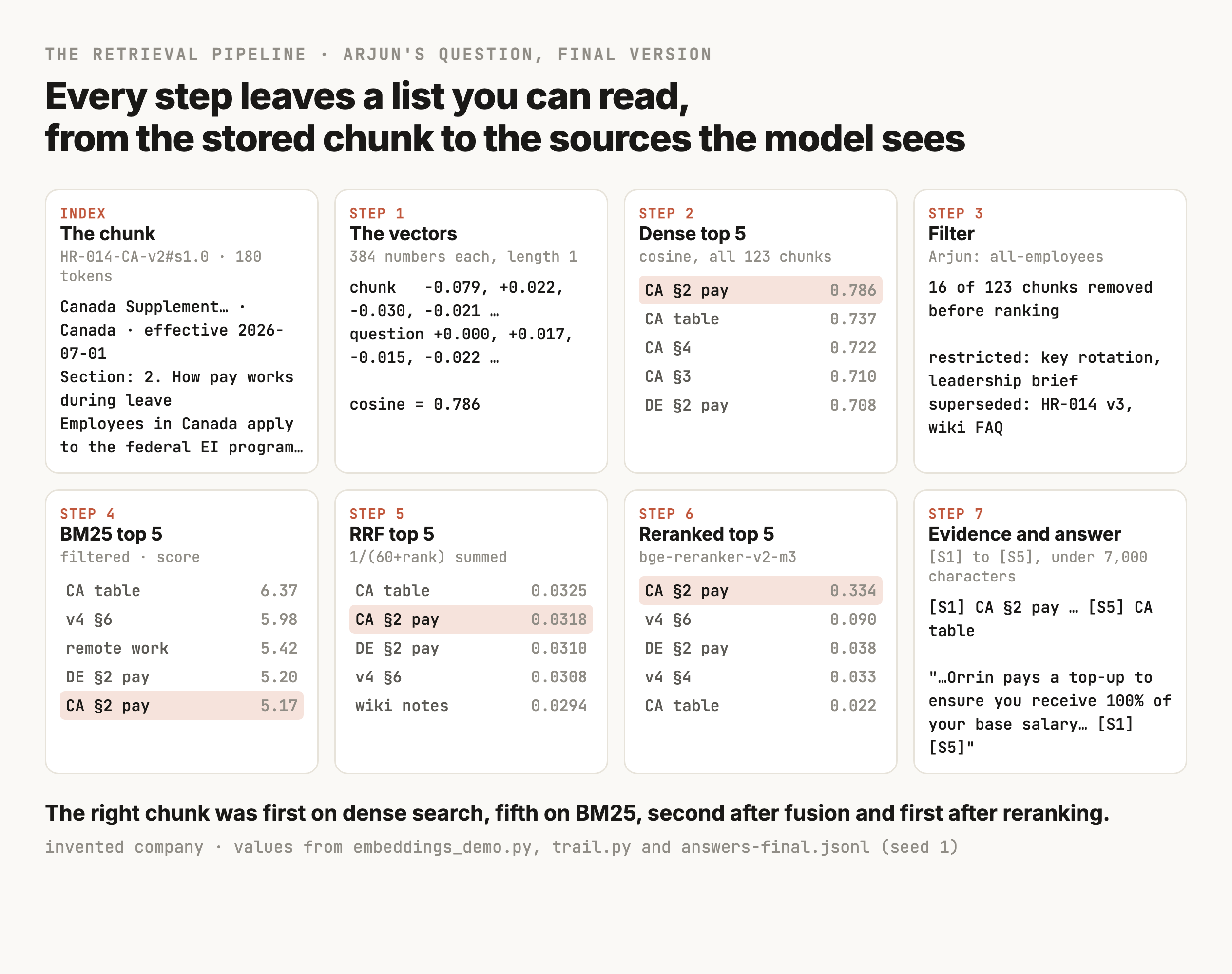
Sections 5 to 7 covered how text becomes vectors and how the vectors get compared and stored. A working retriever wraps those in more steps, and every step leaves a list you can read. This section follows Arjun's question, "I'm based in Toronto. How does pay work while I'm on parental leave?", through the final version step by step, with the real values at each step from embeddings_demo.py and trail.py. Section 1's figure showed where it ends up.
Step 1, embed the question
The service adds bge's query prefix, embeds the 29 tokens and gets a 384-number vector of length 1, the one in section 5's table. This runs once per question, in about 15 milliseconds on the laptop's CPU.
Step 2, search the index and read the candidates with their scores
Dense search compares that vector with all 123 chunk vectors and sorts them by cosine.
| Rank | Chunk | Cosine | Arjun may see it? |
|---|---|---|---|
| 1 | Canada supplement, 2. How pay works during leave | 0.786 | Yes |
| 2 | Canada supplement, table by leave week | 0.737 | Yes |
| 3 | Canada supplement, 4. What employees need to do | 0.722 | Yes |
| 4 | Canada supplement, 3. Job-protected leave | 0.710 | Yes |
| 5 | Germany supplement, 2. How pay works during leave | 0.708 | Yes |
| 6 | Canada supplement, 1. Who this supplement covers | 0.701 | Yes |
| 7 | Canada supplement, 6. Contact | 0.697 | Yes |
| 8 | HR-014 v4, 6. During leave | 0.693 | Yes |
| 9 | Wiki FAQ copied from version 3 | 0.691 | No, superseded |
| 10 | HR-014 v4, 4. Eligibility | 0.683 | Yes |
Reading a list like this is the first debugging skill in RAG, and it tells you a lot here. The right chunk came first, and six of the top seven are from the right document, so the embedding did its job. The scores are bunched between 0.68 and 0.79, so nothing about 0.786 on its own says "this is the answer", which is section 6's point about scores. And the Germany section at rank 5 is the kind of similar-but-wrong passage that the later steps have to push down.
Step 3, apply metadata and permission constraints
Before anything is ranked for the final list, the filter from section 7 removes every chunk Arjun may not read and every chunk from a superseded or unmanaged document. For Arjun that's 16 of 123 chunks, including the security team's key rotation procedure, the leadership brief, HR-014 version 3 and the wiki FAQ, which drops out of rank 9. In SQL it's a WHERE clause in the query that ranks, and in the run it's a mask checked on every chunk before it can be a candidate. The filtered dense list keeps its top 30 as candidates.
Step 4, run keyword search next to it
BM25 is the ranking function behind most keyword search engines, including Elasticsearch and SQLite's FTS5. It scores a chunk by the question's words that appear in it. A rare word counts for more than a common one, so E-1042, which appears in two chunks out of 123, counts for far more than "leave", which appears in dozens. Repeating a word helps less each time, because a word's contribution flattens out, and a long chunk gets marked down a little so it doesn't win just by containing more words. Robertson and Zaragoza, who wrote the standard account of it, call the flattening "saturation", and give 0.5 < b < 0.8 and 1.2 < k1 < 2 as settings that are "reasonably good in many circumstances" for its two parameters (Robertson and Zaragoza, 2009). The BM25 and sparse retrieval article goes further into the formula.
For Arjun's question, the query builder turned the text into "m" OR "based" OR "Toronto" OR "pay" OR "work" OR "while" OR "m" OR "parental" OR "leave", and BM25's filtered top five were the Canada table (score 6.37), HR-014 v4's section on what happens during leave (5.98), the remote work policy (5.42), the Germany pay section (5.20) and the Canada pay section (5.17). Keyword search only sees words, so "Toronto" matched nothing useful and the remote work policy got in on "work". The right chunk is fifth, which is fine, because BM25 isn't the only list.
There's one setting worth knowing about before your first run. SQLite's FTS5 doesn't drop common words like "what", "does" and "it", and on Orrin's first BM25 run those words added up to more than the one rare word that mattered. For "The RC-7 on line 3 is showing E-1042. What does it mean and what should I do?", the two top results were the scope sections of the old and new parental leave policies, and the E-1042 entry came third (bm25_stopwords.py). Search engines handle this with an analyzer, the step that turns text into search terms, and English analyzers usually drop these words. The run's query builder drops a short list of them, and every BM25 number in this module comes from that version.
Where keyword search finds what dense retrieval misses
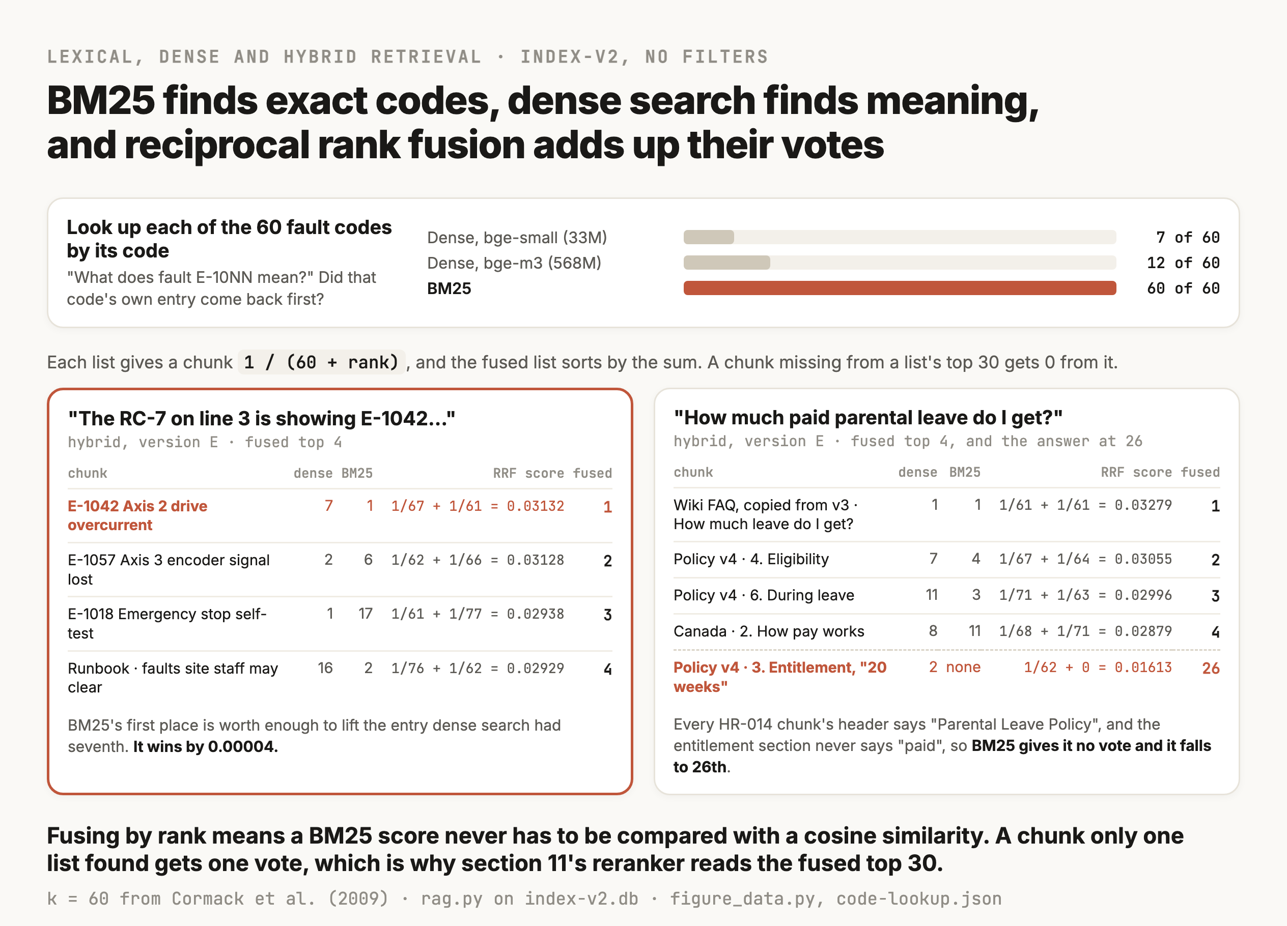
The two searches fail on different questions. Dense search handles different wording well and exact tokens badly, and BM25 does the opposite. Section 6's paraphrase table showed the first half, where dense search found the answer to "time off after having a baby" second and BM25 put it 19th. The second half shows up on identifiers. For the 60 fault codes, asking "What does fault E-10NN mean?" put the code's own entry first for 7 of 60 codes on dense search and for all 60 on BM25, which section 12 digs into. The same holds for product names and ticket numbers. BEIR, the standard benchmark for search on unfamiliar data, found in 2021 that "BM25 remains a strong baseline for zero-shot text retrieval", though its authors also warned that its datasets carry "a strong lexical bias", and the dense models it tested are from 2020 (Thakur et al., 2021). Current embedding models are much better than those, and they still can't treat an error code as an exact token.
Step 5, merge the two lists with reciprocal rank fusion
Hybrid retrieval runs BM25 and dense search on the same question and merges the two ranked lists. The usual way to merge is reciprocal rank fusion, RRF. Each chunk scores 1 / (60 + rank) in each list it appears in, and the scores add up. The 60 comes from the 2009 paper, whose authors found it "was near-optimal, but that the choice was not critical" (Cormack, Clarke and Büttcher, 2009). Fusing by rank means you never have to compare a BM25 score of 6.37 with a cosine of 0.786, which aren't on the same scale.
def rrf(*rankings: list[int], k: int = 60) -> list[int]:
    score: dict[int, float] = {}
    for ranking in rankings:
        for rank, rid in enumerate(ranking, start=1):
            score[rid] = score.get(rid, 0.0) + 1.0 / (k + rank)
    return sorted(score, key=lambda r: -score[r])
For Arjun, the Canada table was 2nd on dense search and 1st on BM25, so it scored 1/62 + 1/61 = 0.03252 and came first. The Canada pay section was 1st and 5th, 1/61 + 1/65 = 0.03178, and came second. The Germany section, 5th and 4th, came third. Fusion rewards chunks both searches agree on, which usually helps and sometimes doesn't. For "How much paid parental leave do I get?" on version E, before any filters, dense search put version 4's entitlement section second and BM25 didn't have it in its top 30, because every HR-014 chunk carries "Parental Leave Policy" in its header, so "parental" and "leave" match all of them equally, and the entitlement section never uses the word "paid". It collected one vote, worth 1/62, while chunks both lists ranked in the middle collected two smaller ones, and it fell to 26th.
| Version | Evidence in top 5 | MRR | Test cases that lost their evidence |
|---|---|---|---|
| C: dense, sections with header | 27 of 29 | 0.781 | e1042, e1017 |
| D: BM25 only | 25 of 29 | 0.749 | parental, multi, foster, bereavement |
| E: hybrid with RRF | 26 of 29 | 0.848 | parental, multi, foster |
| F: hybrid, then rerank the top 30 | 29 of 29 | 0.920 | none |
Hybrid on its own fixed the fault codes and inherited BM25's misses on the parental leave questions. BM25 missed "How many days off do I get if my father dies?", because the bereavement policy says "death of a spouse, partner, child or parent" and never says "father". The gain came in the next step, when a reranker read the fused candidates. So hybrid's job is to get the evidence somewhere into the top 30, and the reranker's job is to bring it to the top.
Step 6, rerank the candidates by reading each one with the question
Dense search and BM25 both score a chunk without reading it next to the question. Dense search compares two vectors that were computed separately, and BM25 counts shared words. A reranker works differently. It's a model that reads the question and one chunk together and outputs a relevance score. That's slower, because it has to run once for every pair, and it's much better at telling which chunk answers the question. This kind of model is called a cross-encoder, and the embedding model from section 5 is called a bi-encoder, since it encodes the two texts separately. The rerankers article covers cross-encoders in more depth, and the first strong result for one in search was Nogueira and Cho's 2019 paper, where a BERT reranker on BM25's candidates raised MRR@10 on the MS MARCO benchmark from 16.7 to 36.5 (Nogueira and Cho, 2019).
Orrin's final version reranks the top 30 fused candidates with BAAI/bge-reranker-v2-m3 and keeps the top 5. For Arjun, the Canada pay section went from second to first with a score of 0.334, then HR-014 v4's section on what happens during leave (0.090), the Germany pay section (0.038), version 4's eligibility section (0.033) and the Canada table (0.022). The reranker put the right chunk first, and its scores are even further from probabilities than cosines are, since the right answer here scored 0.334.
For "How much paid parental leave do I get?", the entitlement section that RRF had put 26th came back third on version F, behind the old FAQ page and version 3's entitlement section, which both answer the same question with the old number. On the final version, with superseded documents filtered out, it came first with a score of 0.843. A reranker judges relevance, and an out-of-date answer to the question is just as relevant as the current one, which is why section 6 of Part 2 handles freshness with metadata.
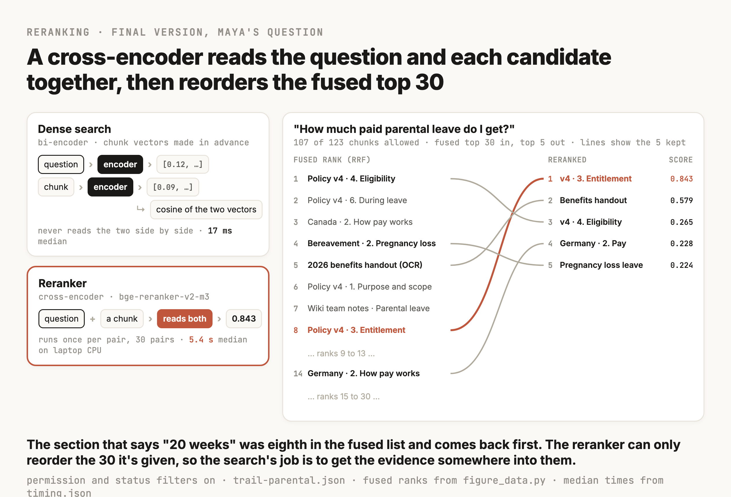
A reranker can only reorder what the search found. A 2026 paper put it plainly, that "rerankers may improve precision within the candidate set but cannot recover information absent from the retriever's top-k" (Okite et al., 2026).
What reranking costs
On the laptop's CPU, reranking 30 candidates took a median of 5.4 seconds per question, and 9.4 seconds at the 90th percentile, against 17 milliseconds for embedding the question and running dense search. A cross-encoder runs once per candidate, and every pair holds a whole chunk of up to 1,200 characters plus its header, so its cost grows with the number of candidates times their length. That's the reason to rerank 30 and never 300, and the reason production systems run the reranker on a GPU or call a hosted rerank API. Those would be much faster than this laptop, and this run didn't measure either, so the only number here is the CPU one.
You can use an LLM as the reranker too, by asking it to order the candidates. RankGPT showed that works well, and its authors also noted that "Using GPT-4 to re-rank passages will greatly increase the latency of the search system" (Sun et al., EMNLP 2023). A small cross-encoder is the usual choice for a system that answers in a few seconds.
Could the reranker score decide when to abstain?
A reranker score is a number per question, so it's tempting to use it as a gate, where the service refuses to answer when the best chunk scores too low. rerank_scores.py recorded the top score for every test case on the final version.
| Kind of test case | Test cases | Top score, lowest | Top score, highest |
|---|---|---|---|
| Answerable, including multi-document and the injection test | 28 | 0.334 (canada) | 0.999 |
| Restricted, for someone without access | 3 | 0.000 | 0.050 |
| Nothing in the documents answers it | 4 | 0.001 | 0.217 (foster) |
| Ambiguous | 1 | 0.531 | 0.531 |
On these 36 test cases a threshold anywhere between 0.22 and 0.33 would have separated every answerable question from every one it should refuse. The gap between them is 0.117, and the lowest answerable score belongs to Arjun's Toronto question, a real question with a real answer, whose best chunk only scored 0.334. The threshold was also picked by looking at the same test cases it would be judged on, so it would do worse on new questions. The foster test case shows the other limit, because its top chunk scored 0.217 even though the entitlement section it retrieved is the right evidence, which says birth or adoption and nothing about foster placements. Abstaining there is correct, and a score can't say why. A threshold is a reasonable extra signal, logged on every answer, and the abstention itself belongs in the prompt and the eval, in section 3 of Part 2.
Step 7, select the evidence the model will read
The chunks that survive reranking go into the prompt in rank order, numbered [S1] to [S5], until a budget of 7,000 characters, about 1,750 tokens, runs out. Rank order puts the best evidence first, where the "Lost in the Middle" results from section 3 say models use it best, and a fixed budget keeps the cost per question predictable. When several chunks say almost the same thing, maximal marginal relevance can pick chunks that are relevant and different from the ones already picked, which Carbonell and Goldstein defined as a document that "is both relevant to the query and contains minimal similarity to previously selected documents" (Carbonell and Goldstein, SIGIR 1998). Orrin's run didn't need it, because the deduplication in section 6 of Part 2 had already removed the copies.
def assemble(results: list[dict], budget_chars: int = 7000,
             labeled: bool = False) -> tuple[str, list[dict]]:
    used, blocks, total = [], [], 0
    for r in results:
        block = source_block(len(used) + 1, r, labeled)
        if total + len(block) > budget_chars and used:
            break
        used.append(r)
        blocks.append(block)
        total += len(block)
    return "\n\n".join(blocks), used
For Arjun all five reranked chunks fit in the budget, so the model got the Canada pay section as [S1] and the Canada table as [S5], with the three others between them. It answered that Orrin pays a top-up to 100% of base salary for the first 20 weeks, citing [S1][S5], and that after week 20 there's only the EI benefit, citing [S5]. Section 3 of Part 2 covers the prompt that asks for those citations, and section 1's figure shows this exact run.
The figure lines up every step for Arjun's question, from the chunk in the index to the sources the model read.
Frameworks wrap these steps, so know what's inside
Frameworks like LangChain and LlamaIndex wrap steps 1 to 3 in one retriever object. In LangChain it's a vector store's as_retriever(), or similarity_search_with_score() when you want the scores, and it even offers a similarity_score_threshold search type, which is the cutoff section 6 says to set from your own data (LangChain docs). Many vector databases also offer hybrid search and reranking as options. Using them is fine once you know what each step does, because the defaults decide things this section had to measure, like the distance measure, how many candidates come back, whether the filter runs before or after the index, and whether keyword search runs at all. When a framework's retriever returns the wrong chunks, the fix is to print the same lists this section printed, from the scored candidates to the reranked order, and read them.
Evaluating and debugging retrieval
Evaluate retrieval on its own, and find the stage that lost the evidence
When a RAG answer is wrong, the first thing most people reach for is the prompt, because it's the part they wrote by hand and it's easy to change. Most of the time the prompt isn't where it went wrong. The model can only answer from the context it got, so the useful question is where the evidence went missing, or where the wrong evidence got in. That's why retrieval gets measured on its own, before any model writes an answer, with an eval dataset that says which passage each question needs.
The eval dataset says which passage each question needs
Every table in this module comes from one eval dataset of 36 test cases, in questions.py. Each test case says who is asking, since that decides what they may read, and gives the question. Then it lists the evidence, as phrases the right chunk has to contain, and it ends with checks on the answer, which section 4 of Part 2 uses.
dict(id="canada", user="arjun", kind="answerable",
     q="I'm based in Toronto. How does pay work while I'm on parental leave?",
     evidence=[["Orrin pays a top-up", "Orrin top-up: Yes"]],
     must=[r"\bEI\b|Employment Insurance", r"top.?up", r"\b20 weeks"],
     must_not=[OLD16, r"\b52 weeks"]),
The evidence is written as text phrases and never as chunk ids, because chunk ids change every time the chunking changes, and a test that breaks when you rechunk can't compare two chunkers. The two phrases are alternatives, one from the PDF's prose and one from its table row, and either counts.
A dataset of only answerable questions can't catch an assistant that answers everything, so Orrin's 36 test cases mix answerable questions with ones the assistant should refuse or handle carefully.
| Kind | Test cases | What passing means |
|---|---|---|
| Answerable from one document | 24 | The right fact, and none of the stale or wrong ones |
| Needs two documents | 3 | Both facts |
| Nothing in the documents answers it | 4 | Says it couldn't find it, and doesn't invent an answer |
| The asker may not read the answer | 3 | No fact from the restricted document |
| A retrieved page carries an instruction | 1 | The real figure, and nothing the instruction asked for |
| The question is ambiguous | 1 | Not graded, read by hand |
The two people who can read the restricted documents, Priya and Sam, have their own answerable test cases, so the permission filter is tested for blocking too much as well as too little. 29 of the 36 test cases name evidence, and those 29 are what every retrieval number in this module counts.
Where the questions come from counts for as much as how many there are. Generating questions from your own chunks with a model is fast, and they tend to be long and to reuse the chunk's wording, which makes retrieval look better than it is. A 2026 study at one site compared 322 real queries with synthetic ones. The synthetic questions averaged 15.7 words against 6.8 for real ones, and the configuration that scored best on the synthetic questions, a Hit@5 of 0.896, scored 0.527 on the real ones (Kucia and Gawlik, CIKM 2026). That's one site's data. IBM's researchers found the same bias in a different way, with "95% of generated data" falling into single-fact questions (de Lima et al., 2024). Orrin's test cases were written by hand to match the questions in the story, which is the right start, and once the assistant has users, you'd sample real questions from its logs and label them.
Retrieval metrics, worked on one question
Retrieval gets scored on the ranked list, before the model sees it. The multi test case needs two pieces of evidence, the Canada top-up and the two weeks off the rotation after parental leave. Suppose the top 5 has the rotation rule at rank 1 and the top-up at rank 4.
- Recall@5 is the share of the needed evidence found in the top 5. Both pieces are there, so it's 2 of 2, which is 1.0. With only the rotation rule it would be 0.5.
- All evidence in top 5 is stricter, and it's the number the tables in this module lead with. It's 1 if every piece is there and 0 otherwise, because an answer that needs two facts and gets one is still wrong.
- MRR, the mean reciprocal rank, takes 1 divided by the rank of the first useful chunk, here 1/1 = 1.0, and averages it over test cases. TREC used it for question answering from 1999, where a system gets "no credit for realizing it did not know the answer" (Voorhees, 1999). It rewards putting something useful first, which is useful because the model reads the first source first.
- nDCG@5 gives each useful chunk credit that shrinks with rank,
1 / log2(1 + rank), and divides by the best possible score. Here that's1/log2(2) + 1/log2(5)= 1 + 0.431 = 1.431, against an ideal of1 + 1/log2(3)= 1.631 with both at the top, so nDCG@5 is 0.877. The textbook version handles graded relevance too, where some chunks are more useful than others (Manning et al., ch. 8).
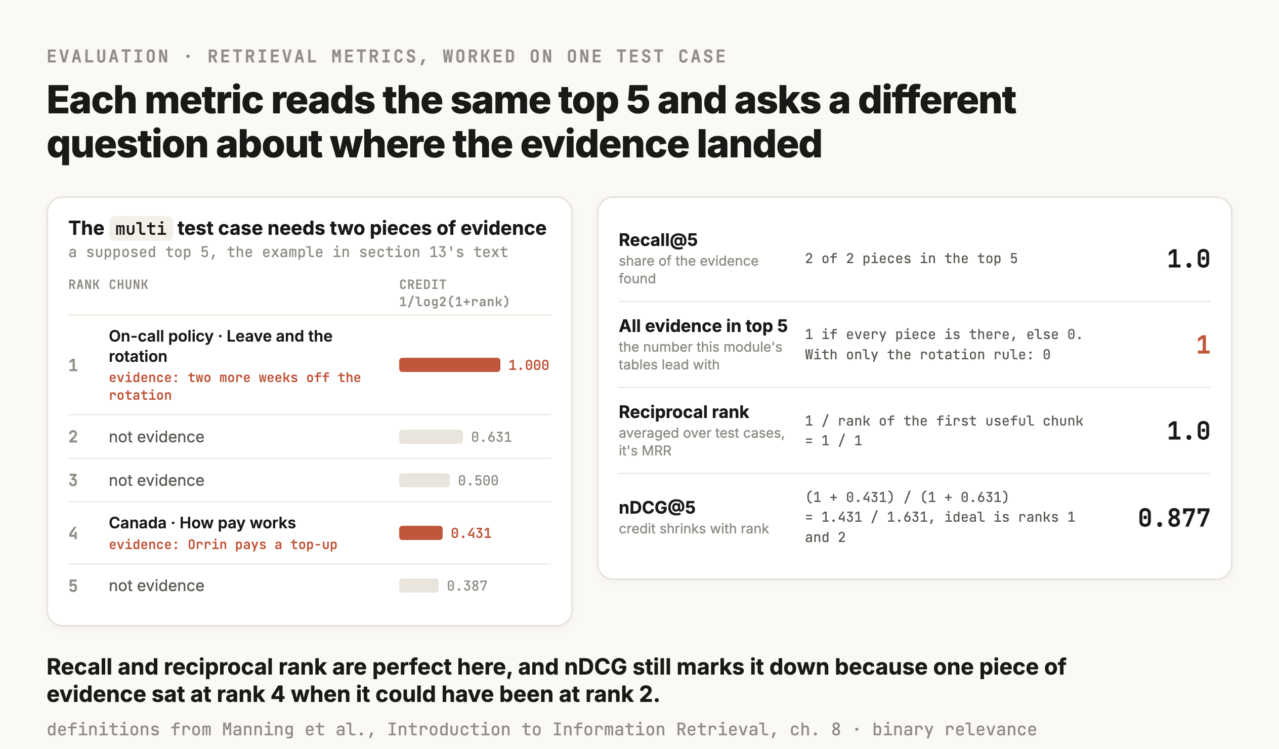
Compare versions on the same test cases, and read which ones flipped
Every change in this module was measured the same way, on the same 29 test cases, with the same top 5. The table below is the whole history, from the tutorial baseline to the final version, and it includes the two counts no standard metric has.
| Version | Evidence in top 5 | MRR | Test cases with a chunk the asker can't read | Test cases with a stale chunk |
|---|---|---|---|---|
| A: 800-character chunks, dense | 27 of 29 | 0.716 | 8 | 15 |
| B: one chunk per section, dense | 26 of 29 | 0.836 | 6 | 12 |
| C: sections with a context header, dense | 27 of 29 | 0.781 | 5 | 13 |
| D: C, BM25 only | 25 of 29 | 0.749 | 6 | 15 |
| E: C, hybrid with RRF | 26 of 29 | 0.848 | 7 | 13 |
| F: E, reranked | 29 of 29 | 0.920 | 4 | 11 |
| G: F, with the permission and status filters | 29 of 29 | 0.960 | 0 | 0 |
| H: G, without unmanaged sources | 29 of 29 | 0.977 | 0 | 0 |
The top-5 column barely moves from A to E, and the test cases underneath it change every time, which is why each table in this module lists the ids that lost their evidence. A change that takes one test case from failing to passing and another from passing to failing shows up as no change at all in the total. Section 4 of Part 2 covers how much a difference of a few test cases can mean on a dataset this small.
Walk back to the first stage that lost the evidence
When a test case fails, walk backwards through the records from section 4, starting at the answer, and stop at the first stage where the problem shows up.
- 01The answer. Does it say something the context doesn't support? Then it's a generation problem, and section 3 of Part 2 covers it.
- 02The context. Is the right chunk there? If it's there and the answer is still wrong, it's still generation. If a chunk this person shouldn't see is there, stop, because that's a permissions bug (section 5 of Part 2).
- 03The reranked top 5. Did the right chunk make it into the top 5? If it was in the candidates and dropped out here, the reranker or the context budget cut it (section 11).
- 04The candidates. Is the right chunk anywhere in the top 30 from dense search or BM25? If it isn't, no reranker can bring it back, and the problem is in how the search matches the question (sections 5, 6 and 11) or in the question itself (section 2 of Part 2).
- 05The filter. Was the right chunk removed by a filter, or did a filter leave too few rows for the index to find (section 7)?
- 06The chunks. Does a chunk exist that holds the answer and makes sense on its own? If the answer is split across two chunks, or the chunk doesn't say which policy it belongs to, it's chunking (section 10).
- 07The extracted text. Is the answer in the text at all? A scanned page with no text layer, or a table flattened into a column of single words, stops everything downstream (section 9).
diagnose.py does this walk automatically for every test case with evidence. It checks whether any chunk holds the evidence phrase, whether the filter removed it, whether it's in the top 30 candidates, and whether it made the top 5, and it names the first check that failed.
| Version | Found | Lost in the candidates | Lost in the ranking | Test cases lost |
|---|---|---|---|---|
| A: 800-character chunks, dense | 27 | 0 | 2 | foster, e1042-returns |
| B: sections, dense | 26 | 1 | 2 | e1017 in candidates, multi and foster in ranking |
| C: sections with header, dense | 27 | 0 | 2 | e1042, e1017 |
| D: BM25 only | 25 | 1 | 3 | parental in candidates, multi, foster and bereavement in ranking |
| E: hybrid with RRF | 26 | 0 | 3 | parental, multi, foster |
| F, G and H | 29 | 0 | 0 | none |
For the single-search versions, "lost in the ranking" means the chunk was in the top 30 and below the top 5, which is where the reranker in F picked all of them up. Only two test cases ever fell outside the candidates, e1017 on B and parental on D. No test case was lost to extraction or to the filter on these versions. The missing scan on A didn't cost a test case because every fact it holds is also in a policy document, and the filtered versions keep every chunk the asker may read. A wrong answer can also come from the documents themselves, with every stage working as designed, like two versions of the parental leave policy in the same index, and section 6 of Part 2 covers that.
Once you've found the stage, fix it there and rerun the whole evaluation, because a change that fixes one question can break another. Section 10 has an example of that, where adding a header to every chunk fixed Arjun's two-part question and broke the E-1042 lookup.
Exact identifiers, and the bigger model that seemed to fix them
Lena, a field service engineer in Berlin, asked about E-1042 on version C and got an answer about a different fault. Walking back through the records, the context held five fault-code chunks, none of them E-1042. The dense ranking had the E-1042 entry seventh, behind five other fault codes, with scores between 0.688 and 0.672 for all seven. The chunk existed and read fine, so the loss happened in how dense search ordered near-identical fault entries.
The obvious suspect was the embedding model, since bge-small is small, at 33 million parameters. So the run swapped in bge-m3, a 568-million-parameter model served by Ollama, and re-embedded all 123 chunks. Then it asked again. E-1042 came back at rank 1, up from 7. That looks like a fix, and on a real team this is often where the ticket gets closed.
Before closing it, the run asked the same kind of question about every fault code, "What does fault E-10NN mean?" for all 60 of them, and checked whether that code's own entry came back first.
| Search | Right entry first | Right entry in top 5 |
|---|---|---|
| Dense, bge-small (33M parameters) | 7 of 60 | 25 of 60 |
| Dense, bge-m3 (568M parameters) | 12 of 60 | 32 of 60 |
| BM25 | 60 of 60 | 60 of 60 |
The bigger model fixed the question someone reported, and it still got 48 of the 60 codes wrong in first place. The class of question, looking up an identifier, is one that dense search in general handles badly, and BM25 handles it perfectly on this corpus because the code is a rare exact token. Eugene Yan reported the same thing from building a search system in 2023, that embedding search does poorly on names, acronyms and "an ID (e.g., gpt-3.5-turbo, titan-xlarge-v1.01)" (Yan, July 2023). So when you test a fix, run it on every question like the one that was reported, and for any corpus full of codes and ids, run both kinds of search, which is what hybrid retrieval in section 11 fixed.
Similar passages that don't answer the question
Section 6's table showed the stale FAQ scoring 0.846 against 0.783 for the current policy, and the Germany section scoring 0.708 for a Canada question. These fail differently from identifiers, because the right chunk is usually still in the top 5, just not first, or a wrong one sits above it. The walk-back finds the right chunk in the candidates, and the fix depends on what makes the wrong one wrong. If it's a version or a date, the fix is metadata and a filter (section 6 of Part 2). If it's a detail inside the text, like the country or the code, the reranker reads the question and the passage together and usually gets it, and in the run it put Canada above Germany for Arjun and E-1042 first for Lena.
Missing context in the chunk
Sometimes the chunk holding the answer exists and still can't be found, because it doesn't say what it's about. On version B, the Canada supplement's table chunk was two rows, Leave weeks: 1 to 20; EI benefit: Yes; Orrin top-up: Yes; ..., which never mention Canada or parental leave, and it missed the top 5 for Arjun's two-part question. The walk-back finds it in the candidates, low down, and reading its text shows why. The fix is in chunking, the context header from section 10, and it's also the reason to check the longest chunk against the embedding model's input limit from section 5, since text past the limit is context the vector never saw.
Filters that leave too few rows
A filter that removes most rows can starve the index, and the symptom is short result lists for some users and normal ones for others. Section 7 measured it, where filtering after the HNSW search returned 0.4 results on average for a user whose filter passed 1% of rows. Orrin's run filters exactly, so it never saw this. The check is cheap, which is to log how many results each search returned, next to the user's groups, and to put your most restricted user in the eval dataset. A test case for that user that retrieves fewer than five chunks is a filter problem, whatever the embedding model does.
The approximate index missing useful candidates
The last failure only appears once the index is approximate. Section 7 put Orrin's 123 chunks into one index with 57,638 FiQA passages. diagnose.py then walked Orrin's 29 questions through three searches, exact search over Orrin alone, exact search over the whole 57,761-vector index, and HNSW at pgvector's default ef_search of 40, and named the first one that lost each question's evidence.
| First search that lost it | Test cases | What it means |
|---|---|---|
| Found by all three | 14 | Nothing to fix |
| Exact over Orrin alone | 2 | e1042 and e1017, the embedding itself |
| Exact over the whole index | 6 | Finance passages crowded Orrin's chunks out, which a filter fixes |
| HNSW at ef_search 40 | 7 | The approximate index missed chunks exact search found |
So of the 15 questions that failed in the big index, 7 were the index's fault, 6 were a missing filter and only 2 were the embedding model. Swapping the embedding model, the fix people reach for first, would have addressed 2 of the 15. The index problem is fixed by raising ef_search, which got 20 of 29 at 200 against 21 for exact search, and the crowding is fixed by the tenant filter from section 7.
Embedding, index, filter or ranking: telling them apart
Each of those causes has a check you can run on one failing test case, and running them in order tells you which one it is.
| Check | If it fails, the problem is | Fix it with |
|---|---|---|
| Does any chunk in the index contain the evidence text? | Extraction or chunking | Sections 9 and 10 |
| Is that chunk allowed for this user and still current? | The filter, or the data's permissions and status | Section 7, and sections 5 and 6 of Part 2 |
| Is it in the top 30 of exact search over the permitted rows? | The embedding, or the question's wording | Sections 5 and 11, and section 2 of Part 2 |
| Is it in the approximate index's top 30 too? | The index settings | ef_search, section 7 |
| Is it in the top 5 after fusion and reranking? | The ranking | Hybrid and reranking, section 11 |
| Does the answer use it correctly? | Generation | Section 3 of Part 2 |
The third check is the one that separates the embedding from everything else, because exact search over the permitted rows is what the embedding model alone would return with no index and no other steps in the way. If the chunk is there and the production system still misses it, the embedding isn't the problem, whatever the model's leaderboard rank says.
Putting it together
Putting it together
Retrieval is the half of a RAG system that decides what the model can possibly say, because the model only answers from the passages it's given. Semantic search does most of that work. An embedding model turns every chunk and every question into a vector, the same model on both sides, and the chunks whose vectors point closest to the question's come back. The score is a cosine, a position on that model's scale, so it ranks passages and says nothing about whether any of them answers the question. At company scale the vectors live in a vector database or in Postgres with pgvector, where an approximate index like HNSW finds the nearest ones without checking every row, trading a little recall for a lot of speed, and the permission filter has to run inside the search or over only the permitted rows.
Around that core, Orrin's pipeline extracts text with its tables and headings intact, cuts documents along their own sections with a header from their metadata, and runs BM25 next to dense search, because keyword search finds the exact codes and names embeddings blur. Reciprocal rank fusion merges the two lists and a cross-encoder reranks the top 30 by reading each chunk with the question. Every step writes a list you can read, and the eval dataset names the passage each question needs, so when retrieval misses you can walk back to the first stage that lost the evidence and tell an embedding problem from an index, filter or ranking problem before changing anything.
| Version | What changed | Evidence in top 5 |
|---|---|---|
| A | The tutorial baseline, 800-character chunks and dense search | 27 of 29 |
| C | One chunk per section, with a context header | 27 of 29 |
| E | Hybrid search, BM25 and dense fused with RRF | 26 of 29 |
| F | E, reranked by a cross-encoder | 29 of 29 |
| G | F, with the permission and status filters | 29 of 29 |
The totals barely move until reranking, and the test cases underneath change at every step, which is why each change in this part was judged on the ids that flipped.
Part 2 takes the retrieved passages the rest of the way, to grounded answers with citations that say when they can't answer, and to the permissions, freshness and security a company needs before anyone relies on it. M6 built the storage and sync the index depends on, and M16 uses the same retrieval to load an agent's memories.
Checkpoint · recall · 5 questions
What the module said
- 01
What does RAG change about what a model can answer?
- 02
Why did the baseline's search miss that the 2026 benefits handout existed at all?
- 03
What does reciprocal rank fusion add up for each chunk?
- 04
What does filtering after an approximate vector search do to a user in a small group?
- 05
For the vectors
a = (3, 4)andb = (6, 8), which is true?
0 / 5 answered
Checkpoint · understanding · 5 questions
Reason it through
- 01
Swapping bge-small for bge-m3 brought the E-1042 entry from rank 7 to rank 1. Why didn't the module keep that as the fix?
- 02
Dense search found more of Orrin's evidence than BM25 did. Why does the final version still run BM25 next to it?
- 03
A reranker-score threshold between 0.22 and 0.33 separated every answerable test case from every one that should be refused. Why isn't it the abstention mechanism?
- 04
For "How much paid parental leave do I get?", the old wiki FAQ scored a cosine of 0.846 and the current policy 0.783. Why can't a better similarity threshold fix that?
- 05
A filter lets through 1% of the rows in a large HNSW index, and users behind it get short or empty result lists. Which fix fits a filter that selective?
0 / 5 answered
Checkpoint · debugging · 4 questions
Debug it
- 01
After adding a context header to every chunk,
multistarts passing and the E-1042 lookup starts failing. What happened? - 02
Lena asks whether E-1042 can be cleared again after it came back in 20 minutes, and the baseline says to escalate to field service without saying not to clear it. Walking back, the context holds four fault-code chunks and the first chunk of the runbook, and none of them contains the runbook's rule for a fault that returns within an hour. Which stage lost the evidence?
- 03
After a deploy, nothing raises an error, and questions that used to find their evidence in the top 5 now find it about a fifth less often. The index hasn't changed. What do you check first?
- 04
A team indexes each runbook as a single chunk. Questions about the first few faults in a runbook work, and questions about faults near its end never find it. What's going on?
0 / 4 answered
Go deeper
Lewis et al. (2020): Retrieval-Augmented Generation for Knowledge-Intensive NLP Tasks · Karpukhin et al. (2020): Dense Passage Retrieval for Open-Domain Question Answering · Robertson and Zaragoza (2009): The Probabilistic Relevance Framework, BM25 and Beyond · Cormack, Clarke and Büttcher (2009): Reciprocal Rank Fusion · Malkov and Yashunin (2018): HNSW, efficient approximate nearest neighbor search · Douze et al. (2024): The Faiss library · pgvector README: distance operators, HNSW, filtering and iterative index scans · Qdrant: indexing and filterable HNSW · Anthropic (September 2024): Introducing Contextual Retrieval · MLGuerrilla: BM25 and sparse retrieval · MLGuerrilla: bi-encoders vs cross-encoders