
The capability
What a classifier is
A classifier takes one input and returns one answer from a list you wrote down before the call, with a number attached saying how sure it is.
The part doing the most work in that sentence is "a list you wrote down before the call". You decide the possible answers in advance, whether that is five support categories, or damaged against fresh, or spam against legitimate, and the component picks among them and can return nothing else. Fixing the answers up front is what makes everything later in this module possible.
The input side is simpler than people expect. It might be a ticket, a photo, twenty seconds of audio or a few seconds of video, and whichever it is, the component reads exactly one of them per call. Nothing about the shape changes when the input does.
What comes back is a score on every label, and that number is the part worth caring about. "Refund, 0.91" is a different object from "Refund", because 0.91 is something your code can compare against a threshold. It is what lets you act automatically on some cases, hand others to a person, and leave the rest alone.
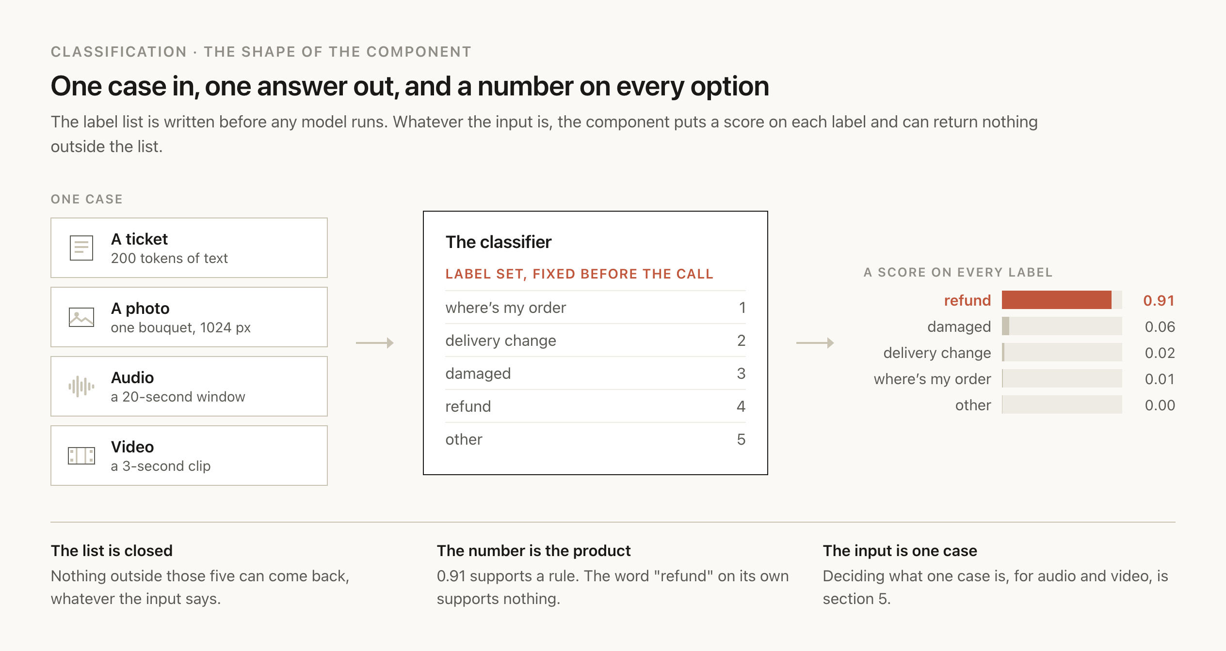
What a classifier cannot do is answer outside the list. If a ticket arrives about something nobody anticipated, what comes back is the closest available label with, if the model is behaving, a low score attached to it. Designing for that case is section 4's job, and it is the reason every taxonomy ends up carrying a bucket for the things you did not think of.
Why this is a capability of its own
Generation leaves the output open. M3 showed a model producing text one token at a time, and M4 then spent a whole section getting that text into a shape your code could parse. A classifier closes the output space before the call even happens, and closing it that early is what pays for everything downstream.
It gives you a number you can threshold, first of all. "Refund, 0.91" supports a rule in a way that "Refund" on its own never will, and a sentence of explanation will not either.
It gives you a confusion matrix, because once the labels are fixed every mistake has a name, in the form of this class predicted when that class was true. Section 7 reads one of those in detail.
It gives you metrics that match the decision you are making, which means precision and recall per class, each weighted by what that class's errors cost you.
And it opens up a much wider choice of models than generation does. For every kind of input, the options run from a hand-written rule up to a frontier model, across four orders of magnitude of cost, and most of those options exist only because the output is closed.
Where it shows up
Classification is the most common job in a production AI system, and it usually runs where nobody sees it.
- A spam filter reading an email and returning spam or legitimate.
- Content moderation reading a post or an image and returning one policy category.
- A defect check on a production line, reading a camera frame and returning pass or fail.
- A wake word detector reading a rolling second of microphone audio and returning heard or not heard.
- A triage step in front of an expensive pipeline, reading a request and deciding which of four handlers gets it. That one is M14, and it's a classifier with cost sitting on the other side of the decision.
Every one of those is the same component, with a different list of labels and a different kind of input. This module builds it once and reuses it.
Where this starts
Three decisions at the flower company
M7 sorted the flower company's support tickets by hand. Someone read 500 of February's tickets and put each one in a bucket, which is how the framing page came to say that 45% are "where's my order", 15% are delivery changes, 20% are damaged or wilted flowers, 10% are refunds and charges, and 10% are everything else. That sort is what justified building the agent, because 60% of those tickets need no model at all.
None of that sorting happens on live traffic. Every ticket still arrives in one queue, and the agent reads all of them, including the 45% that a tracking link answers and the 15% that a change form handles.
The same company has two more decisions to make, and neither of them is text.
The first is a photo. M7's plan for v2 has the customer sending a picture of the bouquet, and something has to decide whether it arrived damaged before a refund goes out.
The second is a phone call. The company takes about 4,000 of those a month, four minutes each on average, and every one gets picked up by whoever is free. The same five buckets apply to them as to tickets, and nobody knows which bucket a call belongs in until a person has sat and listened to the whole thing.
All three are the component from section 1, with a different kind of input each time. This module builds all three, and they stay the running example to the end.
What changes between a ticket, a photo and a call is narrower than it looks. The label set, the metrics, the thresholds, the calibration and the drift monitoring are the same work in all three, which is why this module teaches them once. Two things do change. Which models can read that kind of input, and what counts as one input in the first place. A ticket is obviously one input. A four-minute call is a file, or a twenty-second window, or a stretch of speech between two pauses, and choosing among those three changes your labels, your metrics and your bill.
The temptation in all three is to reach for a prompt, since that is the tool everybody has. A prompt does work here, and it sits near the top of a ladder this module climbs four times, which is to say it is the most expensive option on every one of those ladders.
The company is made up, and so are its numbers.
The component
The seam every option sits behind
Section 6 lists about twenty ways to build this thing, from a regular expression to a frontier model. They all sit behind one function, which is what lets you swap one for another without touching the code that acts on the answer.
LABELS = ["wheres_my_order", "delivery_change", "damaged", "refund", "other"]

def classify(case) -> dict:
    """`case` is a ticket body, a photo, or twenty seconds of audio.
    Returns {"label": str, "scores": {label: float}} over LABELS."""
    ...

result = classify(ticket.body)
if result["scores"]["refund"] >= 0.80:
    route_to(refund_queue)
elif max(result["scores"].values()) < 0.50:
    route_to(human_triage)          # section 8
else:
    route_to(handler_for(result["label"]))
M4 put every model call behind one complete() function. This is the same idea for a different job, and it's why swapping a prompt for a trained model later is a contained change.
A prompt can do this job. M4's structured output makes the shape reliable, so {"label": "refund"} comes back as JSON on every call. The number beside it is a different matter. If you also ask the model for a confidence, the characters 0.91 get generated the same way the word refund does, and nothing in the decoding loop checks them against how often the model turns out right. Xiong and colleagues benchmarked the confidence five models state in words, across five kinds of dataset, and found they "tend to be overconfident" (Xiong et al., 2023). An LLM prompt is a classifier with a soft score, which carries a routing decision fine and starts costing you in section 8.
Taxonomy
The label set is the design
Most of the problems people bring to a classifier turn out to be problems with the labels, and no amount of model selection fixes those. Before any of section 6's options is worth weighing, five decisions have to be made and written down somewhere.
The first is whether a case gets one label or several. A ticket saying "my flowers arrived wilted and I want my money back" is both damaged and refund, so either the taxonomy allows more than one label per ticket, or a written rule decides which one wins. The flower company picks one label per ticket, with damaged beating refund, on the grounds that the photo check has to happen first anyway.
The second is what "other" means. Every taxonomy needs somewhere to put the thing it did not anticipate, and that bucket is where new classes come from, so treating it as a dumping ground wastes the one signal it carries. M7's "other" was 10% of tickets, and section 9 comes back to what you do with it.
The third is a written definition for each label, including the edge cases. "Delivery change" means the customer wants a different date, address or time window for an order that has not shipped yet, and a change requested after delivery is a refund. Two sentences per label does it, as long as they are followed by the cases that nearly went the other way.
The fourth is who does the labelling and how you know they agree with each other. Getting two people to label the same 100 tickets and comparing the results is the cheapest quality measurement in this whole module. If they disagree on 18 of the 100, those 18 tickets are where a definition is unclear or a labeler slipped, and each one needs a reviewed label before it goes into the dataset.
The fifth is what each label is for. A label exists because something different happens next, so if two of them lead to the same handler, you have one label until the handlers diverge.
All five decisions belong in one document that somebody maintains, since five people's memories of them will drift apart. An entry in it looks like this:
| Field | Refunds and charges |
|---|---|
| What it covers | The customer wants money back, disputes a charge, or was billed twice |
| What it excludes | Damaged flowers, which take the damaged label so the photo check runs first |
| Edge case | "I was charged for two bouquets and only got one" is a refund, since no photo decides it |
| Edge case | "Cancel my order" before it ships is a delivery change, since no money has moved |
| What happens next | The refund queue, where a person approves anything over $50 |
Agreement gets measured on an overlap. Two people label the same 100 tickets without seeing each other's answers, and you count how often they match. Raw percent agreement is the number to start with, and Cohen's kappa adjusts it for the matches two people would hit by chance, which counts for a lot when one class is 45% of traffic. Agreement measures how consistent two labelers are with each other, which is a different quantity from how often either of them is right. Take a yes/no question like refund or not refund, and two labelers who are each right on 90% of tickets and make their mistakes independently. They match when both are right, which happens 0.9 × 0.9 = 81% of the time, and they also match when both are wrong, since on a yes/no question two wrong answers are the same answer, which happens 0.1 × 0.1 = 1% of the time. That's 82% agreement from two people who are each 90% accurate. A model trained on thousands of their labels could end up more accurate than either of them, because their mistakes land on different tickets and the model learns the pattern most of the labels agree on.
Low agreement limits the score you can read. If each test label came from one of those labelers, one label in ten is wrong, so a model that got every ticket right would still score about 90% against them, and a real improvement past that point wouldn't show up in the number.
So the disagreements get reviewed before the labels are used. Every ticket the two people label differently goes to a third person, or back to the two of them together, and they decide the label against the annotation guide. The test split uses only reviewed labels. Some disagreements turn out to be a slip, and the reviewer corrects it. Others are a ticket the guide doesn't cover, like an address change on an order that already shipped, and that one becomes a new edge-case row in the guide before the affected tickets get re-labeled. A ticket where both labels stay defensible after review gets marked as ambiguous and left out of the test split's headline number, because neither answer on it can be scored as the right one.
M1's discipline carries over with no changes. The labeled tickets are a dataset, they get split into train and test, the test split never trains anything, and every ticket the classifier gets wrong in production is a candidate for the dataset.
Segmentation
What counts as one case
A classifier takes one input and returns one answer. Deciding what that one input is happens before any model gets chosen, and for anything with a time axis it's the hardest decision in the module.
Text and images mostly answer the question for you. One ticket is one input, one photo is one input, and there is not much to argue about. Audio and video leave the decision open, and you have to make it.
The four-minute phone call could be any of three things:
| The case is | How many per call | What a label means | Fits when |
|---|---|---|---|
| The whole file | 1 | This call was about a refund | The decision waits until the call ends |
| A fixed window, say 20 seconds | 12 | This 20 seconds sounds like a refund | The decision has to happen while the caller is still talking |
| A speech segment between pauses | Varies, often 15 to 40 | This utterance was about a refund | The answer lives in one sentence somewhere in the call |
Picking one of those three changes four things downstream, which is why it is worth deciding deliberately.
It changes what your labelling costs. One label per call is cheap to collect, because a person listens and picks a bucket. Window labels need somebody marking start and end times, which is slower per hour of audio and produces about twenty times as many examples from the same recordings.
It changes what your metrics mean. 90% per window and 90% per call are different numbers coming off the same model, since a call cut into twelve windows can have four of them wrong and still land on the right bucket once you combine them. Section 7 has that arithmetic.
It changes your latency, and this is usually the one that decides it. A file-level classifier cannot answer until the file exists, whereas a window-level one has an answer twenty seconds in, which is the difference between routing a live caller and tagging a recording after the fact.
And it changes the bill. The flower company's 4,000 calls come to 16,000 minutes a month. Priced per minute that is one number, and priced per window it is 48,000 separate decisions.
One rule resolves most of it, which is to label at the level the decision gets made at. If the product routes a live call, the case is a window. If the product tags recordings for a weekly report, the case is the file.
Video is the same question with a frame rate
Video hands you the choice as a number. A packing-line camera watching whether bouquets get wrapped correctly runs 8 hours a day, 22 days a month, and how often you look at it is the entire cost story:
| Sampling | Frames a month |
|---|---|
| Every frame at 30 fps | 19,008,000 |
| One per second | 633,600 |
| One every 5 seconds | 126,720 |
| One every 30 seconds | 21,120 |
Multiply any row by your cost per frame. A hosted vision model at even a tenth of a cent per image makes the top row absurd and the bottom row fine, which is why production video classification almost always runs a small model on hardware you own, where the per-frame fee is zero and the frame rate is bounded by the GPU alone.
The other half of the video question is whether a label belongs to a frame or to a clip. "Is a person in shot" is a frame label. "Did the wrapping get done correctly" is a clip label, because it takes several seconds of motion to tell. A frame classifier can't answer a clip question no matter how many frames you feed it one at a time, and that's the point at which you need a model that reads a stack of frames together.
The ladder
Pick the option your data can support
Four questions decide which option fits, and none of them is about which model is best:
- 01How many labeled examples do you have today?
- 02How often does the label set change?
- 03Can the data leave your systems?
- 04How many decisions a day, and how fast does each one have to be?
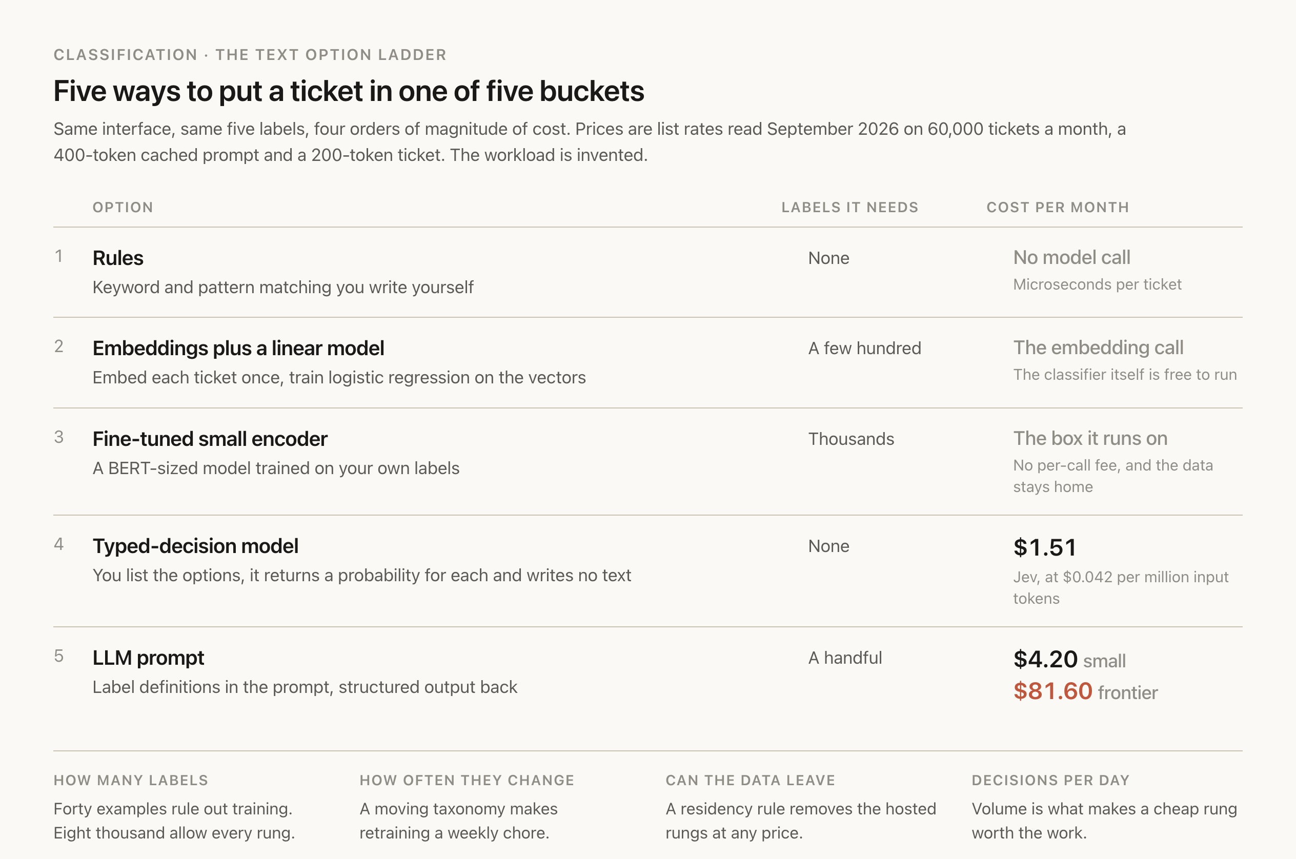
The costs are computed on 60,000 tickets a month with a 400-token cached prompt and a 200-token ticket, at list prices read in September 2026, and the workload is invented. What to take from the column is the ratio, since the frontier prompt costs about 54 times the typed-decision model for the same decision.
Text
Rules get dismissed faster than they deserve. A ticket containing a 5-digit order number and the word "where" is a where's-my-order ticket, and you can decide that with no model at all, in microseconds. What rules cannot survive is paraphrase, which is why they work best as a first pass that handles the obvious cases and hands everything else down the ladder.
Embeddings plus a linear model is the rung people forget exists. Each ticket becomes a vector once, and logistic regression over a few hundred labelled vectors trains in seconds on a laptop. After that the classifier itself costs nothing to run, and the embedding model is the only outside dependency you are carrying. M19 covers embeddings properly in the context of retrieval, and the same vectors work here without modification.
A fine-tuned encoder is the answer when the data cannot leave your network and the volume is high enough to justify the work. It is a training job, which M21 covers in its own right, and of everything on this ladder it demands the most labels and the most settled taxonomy before it pays off.
A typed-decision model is the newest rung here, and it did not exist when most of this advice was written. Jev, from TypeSafe, takes a question whose possible answers you list in advance and returns a probability for each one, and it never writes any text at all. TypeSafe prices it at "$0.042 / MTok ($42 per billion tokens)" with output tokens free, and claims 70 to 500 milliseconds per call (TypeSafe's launch post). Those speed and quality numbers are the vendor's own, measured against reference answers the vendor chose, so they're worth confirming on your own tickets. What the shape buys you is real regardless: a probability per label, with no training, and a label set you can edit by changing the request. The Jev article goes through the model itself.
An LLM prompt is worth its cost when you have five labelled examples and not five hundred, when the taxonomy is still moving every week, or when the label depends on something only a person reading carefully would catch. It is also the fastest way to produce your first labelled thousand tickets, which is how most teams end up affording the cheaper options below it.
Images
The damaged-bouquet check is a two-class decision on a photo, and the same four questions apply to it.
| Option | What it is | Labels it needs | Fits when |
|---|---|---|---|
| Zero-shot CLIP or SigLIP | Embed the image, compare it against embedded label phrases like "a photo of wilted flowers" | None | The classes can be described in words |
| Frozen features plus a linear model | Embed with a self-supervised backbone like DINO, train logistic regression on the vectors | A few hundred | One visual domain, stable classes |
| Fine-tuned image classifier | Train a vision transformer on your labels | Thousands | High volume, on-device, or data that can't leave |
| A vision-language model | Ask a multimodal model the question directly | A handful | The answer needs context, or reading text in the image |
| Detection | YOLO or Grounding DINO, when the answer is a location or a count | Hundreds, with boxes | "How many stems are broken" is a different question from "is this damaged" |
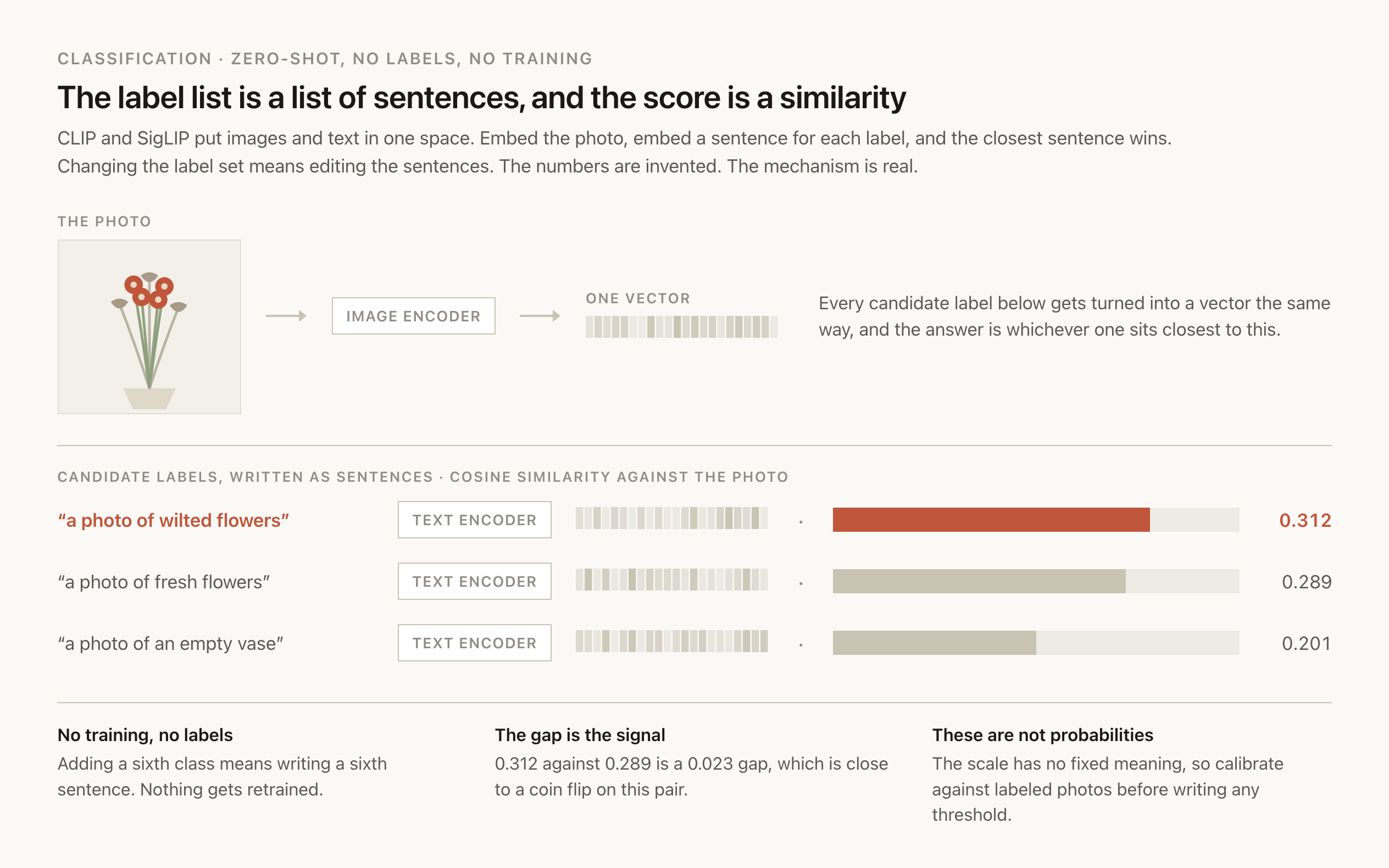
Zero-shot is worth trying first because it costs a morning. CLIP's paper reports matching "the accuracy of the original ResNet-50 on ImageNet zero-shot without needing to use any of the 1.28 million training examples it was trained on" (Radford et al., 2021). That's a general claim on a general benchmark, and wilted roses against fresh ones is a narrower question, so it may do better or much worse. You find out by running it on a hundred labeled photos, which is the same test any other rung gets.
Two things are worth watching out for with images in particular. The first is that a similarity score from CLIP or SigLIP is not a probability, which makes the calibration check in section 8 carry more weight here than anywhere else in the module. The second is that the question you have been handed is often a detection question in disguise, and no amount of classifier accuracy will answer it.
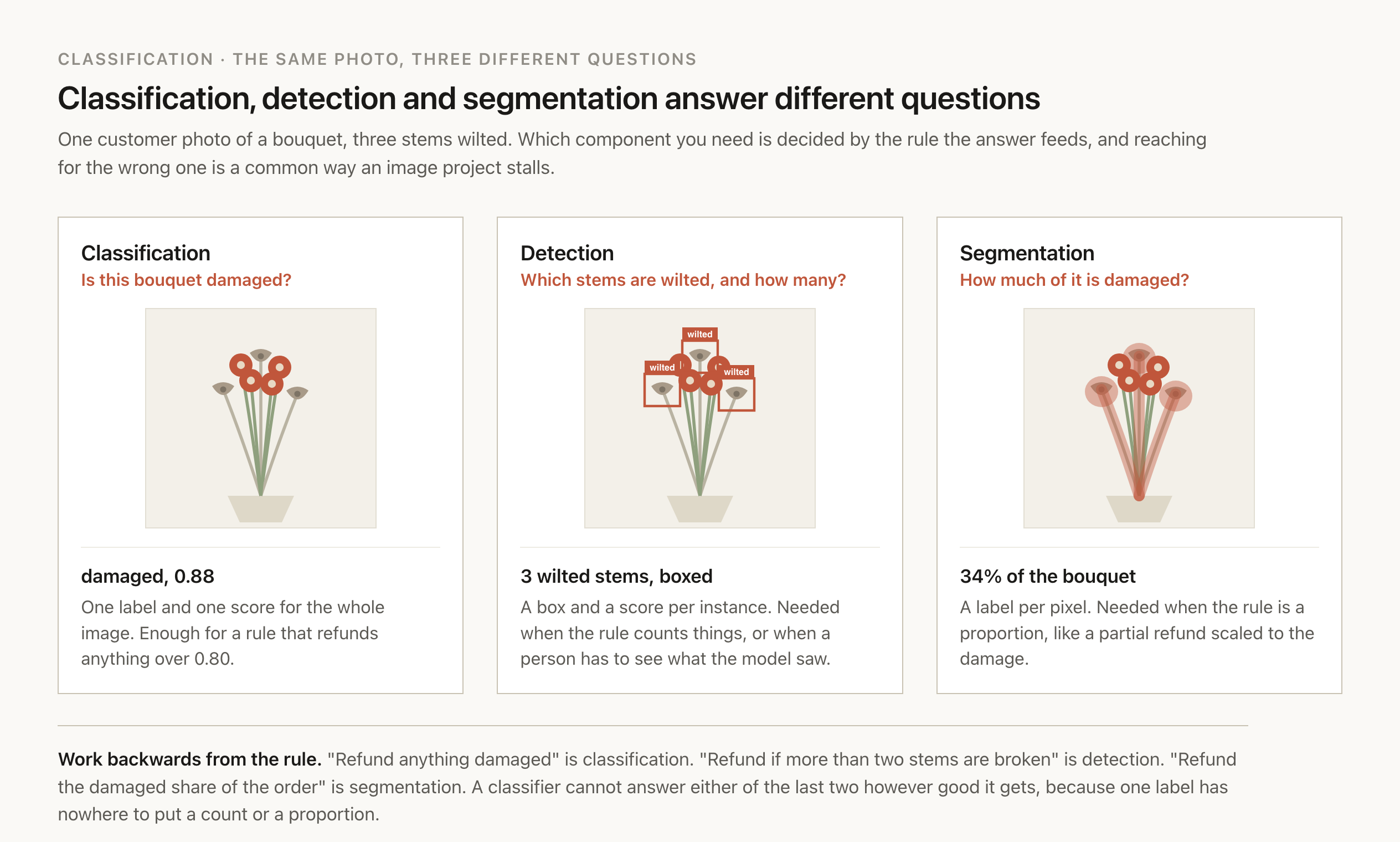
Work backwards from the rule the answer feeds. "Refund anything damaged" is a classification question. "Refund if more than two stems are broken" is a counting question, so it needs detection. "Refund the damaged share of the order" is a proportion, so it needs segmentation. The CLIP, SigLIP, DINO and YOLO articles cover the models, M20 goes deeper on vision-language models, and M21 covers the training runs.
Audio
The phone line has the same five buckets and a different ladder, and the first rung is the one most teams reach for without weighing it.
| Option | What it is | Labels it needs | Fits when |
|---|---|---|---|
| Transcribe, then classify the text | Speech recognition, then any rung from the text ladder | Whatever the text rung needs | The answer is in the words, and you can wait for a transcript |
| Zero-shot CLAP | Embed the audio, compare it against embedded label phrases | None | The classes can be described in words, including non-speech sound |
| Frozen speech features plus a linear model | Embed with wav2vec 2.0 or similar, train logistic regression on the vectors | A few hundred clips | Tone, speaker or acoustic classes, with little labeled audio |
| Fine-tuned audio classifier | Train an Audio Spectrogram Transformer on your labels | Thousands of clips | High volume, on-device, or audio that can't leave |
| An audio-native LLM | Send the audio to a multimodal model and ask | A handful | The answer needs reasoning over what was said |
Transcribe-then-classify is what most teams build first, and the cost of it lands somewhere people do not expect. Transcribing 16,000 minutes a month at gpt-4o-mini-transcribe's $0.003 a minute costs $48.00. Classifying those transcripts on a small model costs $0.88 (OpenAI pricing, read September 2026). Getting to text is 98% of the bill, so the lever is the transcription model, and gpt-live-transcribe at $0.017 a minute would take the same job to $272.00.
The rungs that skip text exist for two reasons. One is that some labels aren't in the words at all. An angry caller and a calm caller can say identical sentences, and only the audio carries the difference. The other is latency. Transcription has to wait for the speech to finish. A classifier reading the first twenty seconds of audio can route a live caller while they're still talking.
Zero-shot audio works the same way zero-shot images do. CLAP embeds audio and text into one space, and its authors report that it "achieves state-of-the-art performance in the zero-shot setting" for audio classification (Wu et al., 2022). As with CLIP, that's a benchmark claim, and your hundred labeled clips decide whether it holds for your classes.
Frozen speech features are the audio version of the workhorse rung. wav2vec 2.0 learns speech representations without labels, and its paper reports usable recognition from "just ten minutes of labeled data and pre-training on 53k hours of unlabeled data" (Baevski et al., 2020). The same representations feed a linear classifier trained on a few hundred of your clips.
A fine-tuned audio classifier is the high-volume answer. The Audio Spectrogram Transformer was "the first convolution-free, purely attention-based model for audio classification", reporting 95.6% on ESC-50 and 98.1% on Speech Commands V2 (Gong et al., 2021). Those are benchmarks of everyday sounds and short spoken commands, so they say the architecture works, and nothing about your classes.
Video
Most video classification is image classification with a sampling policy bolted on, and saying so out loud saves a lot of work. Sample frames, run an image classifier, combine the per-frame answers, and you have a video classifier. That covers every label a single frame can carry.
| Option | What it is | Fits when |
|---|---|---|
| Sample frames, classify each one | Any rung from the image ladder, plus a rule for combining frames | The label is visible in one frame |
| Sample frames, classify with a VLM | Send a handful of frames to a multimodal model | Few labels, and the answer needs context across shots |
| A clip model | VideoMAE or similar, reading a stack of frames together | The label lives in the motion |
| Detection plus tracking | Detect per frame, link the boxes over time | The answer is a count, a path or a duration |
The line that decides between the first two rows and the third is whether the label survives a still frame. "Is the workstation occupied" survives. "Did the wrapping get done correctly" doesn't, because it's a sequence. Clip models read frames together for exactly that reason, and VideoMAE's authors report 87.4% on Kinetics-400 "without using any extra data", alongside a finding worth carrying into your own run, that "data quality is more important than data quantity" for this kind of pre-training (Tong et al., 2022).
The pattern that repeats
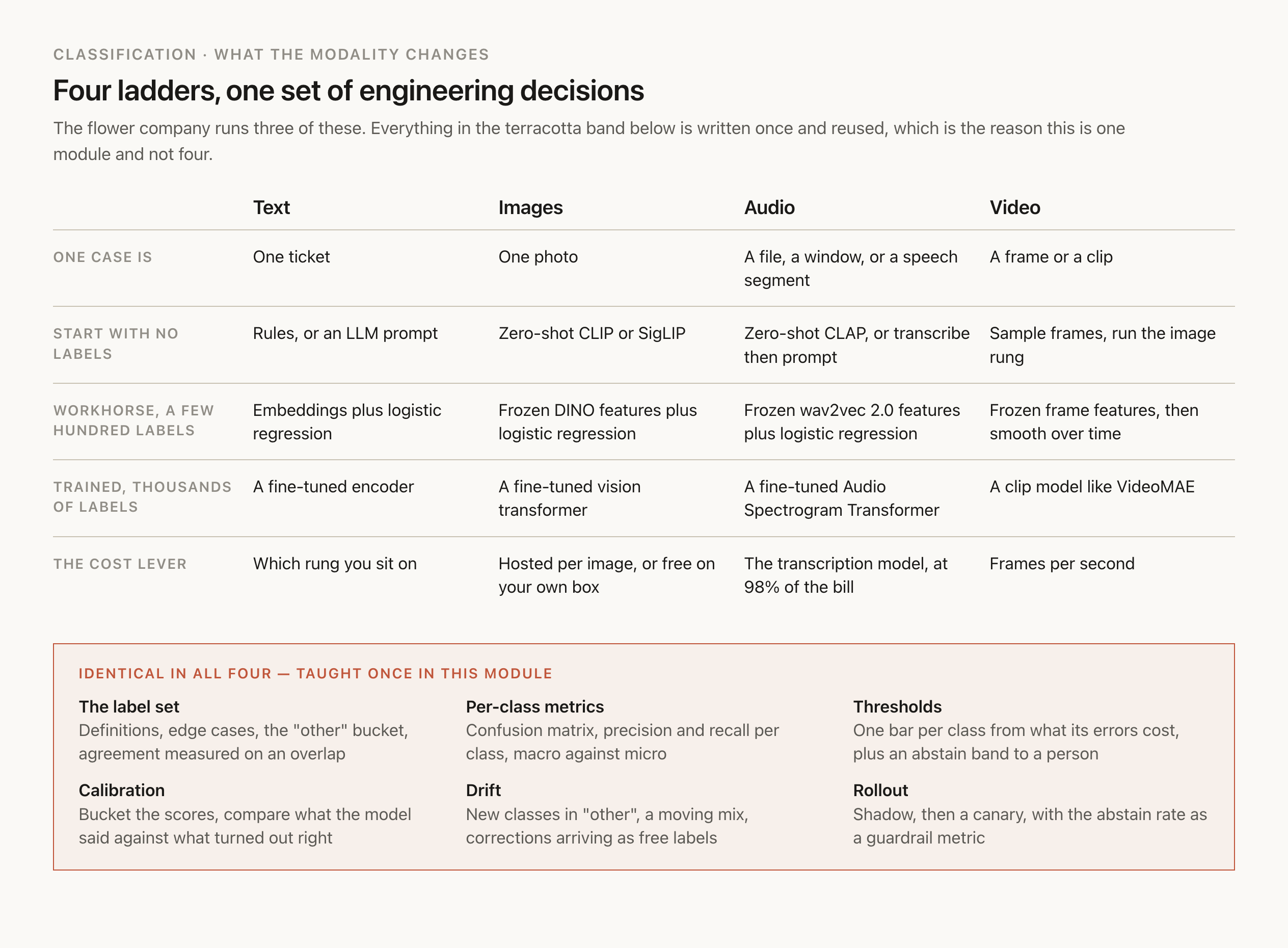
Four ladders, one shape. Every one of them starts with something that needs no labels, ends with something that needs thousands, and puts a hosted general-purpose model somewhere near the expensive end.
So the play is the same in all four. Start at the zero-label rung to find out whether the problem is easy. Use a prompt or a zero-shot model to produce the first labeled thousand examples. Then move down the ladder once the labels exist and the taxonomy has stopped moving, because the cheap rungs are cheap in exactly the way that compounds, with no per-call fee and a latency floor set by your own hardware.
Metrics
Accuracy hides the errors that cost you
The flower company builds the classifier, runs it on a held-out 2,000-ticket test split, and gets 87.2% accuracy. A model that answers "where's my order" every single time gets 45%, because that's the biggest class. So 87.2% says the model beats the dumbest possible baseline, and nothing else.
The matrix says the rest:
| True label | Where's my order | Delivery change | Damaged | Refund | Other |
|---|---|---|---|---|---|
| Where's my order (900) | 855 | 30 | 5 | 0 | 10 |
| Delivery change (300) | 45 | 240 | 0 | 3 | 12 |
| Damaged (400) | 8 | 2 | 360 | 20 | 10 |
| Refund (200) | 3 | 2 | 35 | 150 | 10 |
| Other (200) | 25 | 15 | 12 | 8 | 140 |
Read across a row for recall, which is the share of that class the model found. Read down a column for precision, which is the share of that prediction that was right.
| Class | Precision | Recall | F1 |
|---|---|---|---|
| Where's my order | 91.3% | 95.0% | 93.1% |
| Delivery change | 83.0% | 80.0% | 81.5% |
| Damaged | 87.4% | 90.0% | 88.7% |
| Refund | 82.9% | 75.0% | 78.7% |
| Other | 76.9% | 70.0% | 73.3% |
Two averages summarize that table and they disagree on purpose. Macro averaging treats every class the same, so it comes to 83.1% here. Micro averaging pools every decision, which for single-label classification equals accuracy, 87.2%. The gap between them is the imbalance, since the big easy class is carrying the micro number. scikit-learn exposes both as f1_macro and f1_micro, and picking one is a decision about whether a rare class counts as much as a common one.
Now price the errors, which is where M7's failure ladder comes back. The 50 refund tickets the model missed become customers waiting on money nobody is working on, which M7 rated near the top of its cost ladder. The 45 delivery changes sent to the where's-my-order handler get a tracking link and write in again, costing a second contact. Same-sized errors, different costs, so the targets per class aren't the same number.
That's the sentence to take into an interview. A classifier's quality bar is one line per class, written from what that class's mistakes cost, and a single accuracy number can't express it.
Everything in this section is modality-blind. A confusion matrix over damaged and fresh bouquets reads the same way, and so does one over call windows. The only thing to watch is what the rows are counting. If the case is a 20-second window, the matrix counts windows, and a model at 88% per window is not a model at 88% per call. Report both, and be explicit about which one the ship bar refers to.
Thresholds and abstention
Turn scores into decisions
The model returns a probability per label. What the product does with it is a separate decision, and it's where most of the value is.
Take the refund class, and vary the threshold above which a ticket is routed to the refund queue:
| Threshold | Precision | Recall | Share of tickets flagged |
|---|---|---|---|
| 0.30 | 44.8% | 98.5% | 22.0% |
| 0.50 | 70.6% | 86.5% | 12.2% |
| 0.70 | 90.8% | 54.0% | 5.9% |
| 0.90 | 100% | 11.5% | 1.1% |
Those come from an invented score distribution, and the shape is what every threshold table looks like. Raising the bar buys precision and pays for it in recall. There's no threshold that's right in general, only one that's right given what a false positive and a false negative each cost.
The third option is to not answer
M9 gave the agent a coverage check, where it declines to answer below a cutoff and hands the conversation to a person. A classifier can do the same thing, and it turns a single threshold into a band:
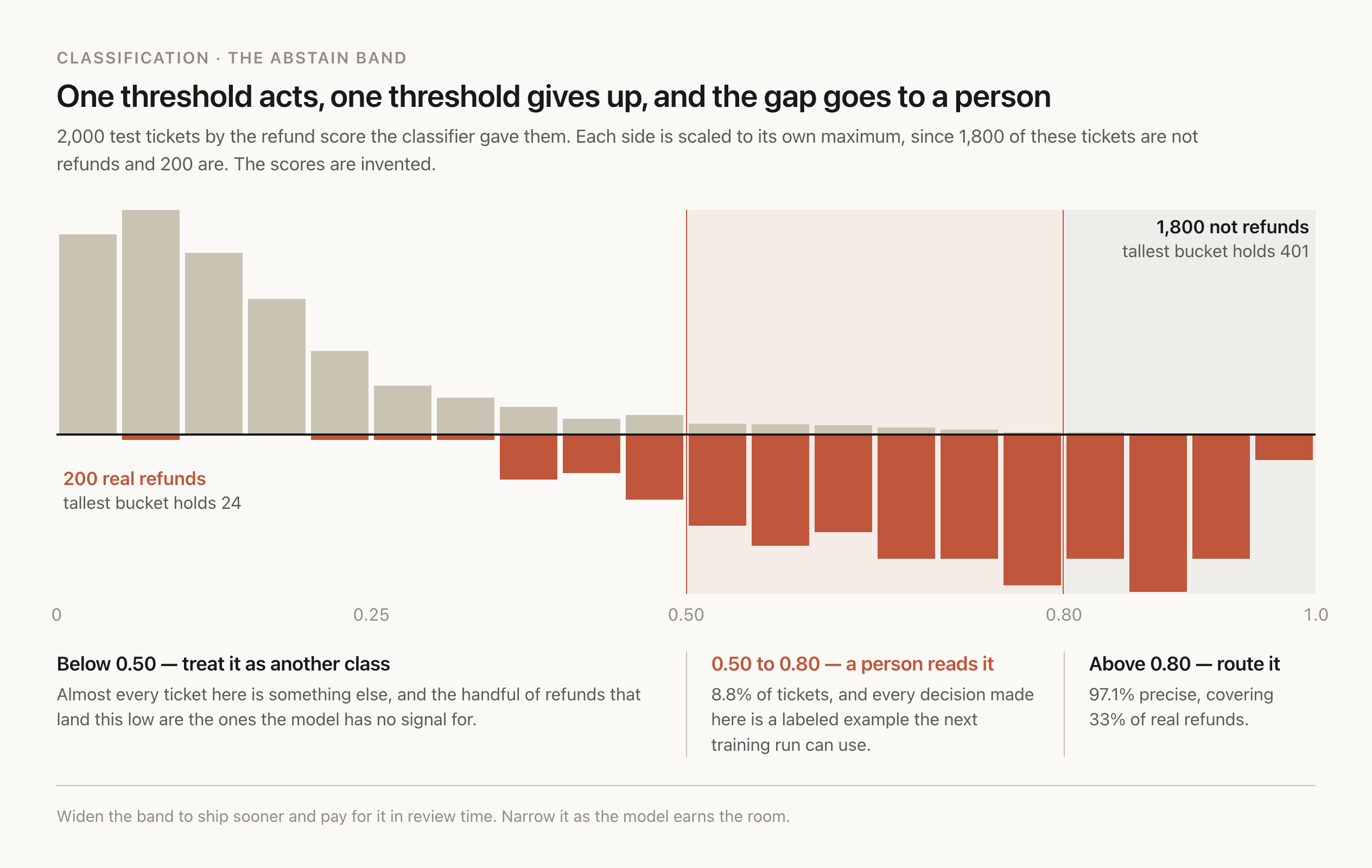
- Above 0.80, route automatically. On this distribution that's 97.1% precise and catches 33% of real refunds.
- Below 0.50, treat it as another class entirely.
- Between the two, send it to a person. That's 8.8% of tickets, and the people looking at them are producing exactly the labels the next training run needs.
An abstain band is how a classifier ships before it's good enough to ship. You start with a wide band and narrow it as the model earns the room.
A score per window needs collapsing
When the case is a window, the model hands you twelve scores for one call and the product needs one answer. How you collapse them is a decision with its own failure modes:
You could take the maximum, which lets one confident window decide the whole call. That catches a refund mentioned once in passing, and it also means a single false positive anywhere in four minutes routes the entire call wrong.
You could take the mean, which is far more stable and buries exactly the case the maximum was good at, since a request raised once across twelve windows barely moves an average.
Or you could require two windows in a row above 0.70, which turns out to be a different and usually better detector than any single window above 0.70. Noise rarely repeats itself in consecutive windows, and a topic somebody is genuinely discussing does.
The same three choices appear in video as temporal smoothing across frames, for the same reason. A per-frame classifier that flickers between labels on consecutive frames is reporting noise, and requiring agreement across a few frames removes most of it without touching the model.
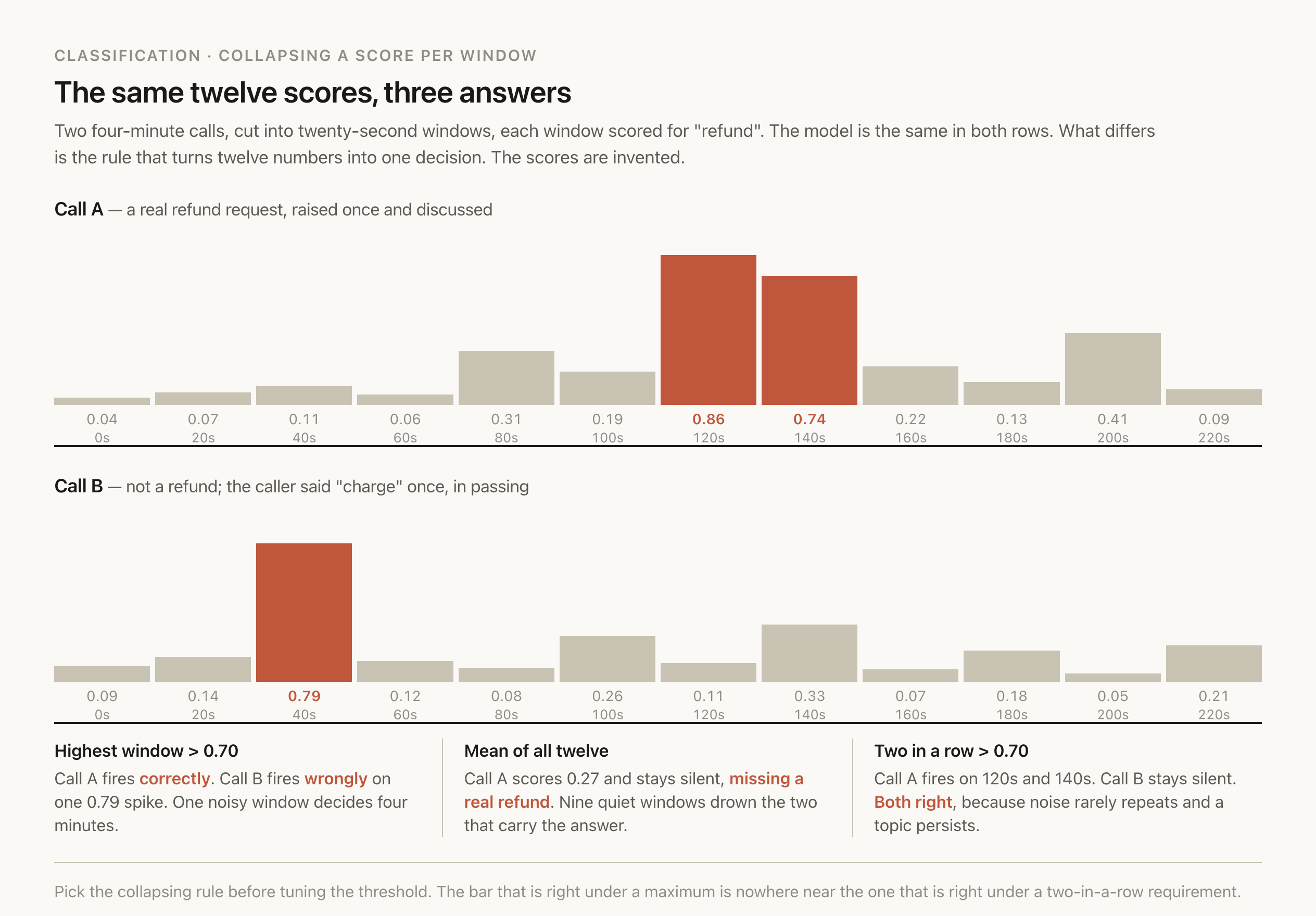
Pick the rule before tuning the threshold, since the threshold that's right under a maximum is nowhere near the one that's right under a two-in-a-row requirement.
Scores aren't probabilities until you check
A model's output looks like a probability and often isn't one. Guo and colleagues measured this on image classifiers and put it plainly, that "modern neural networks, unlike those from a decade ago, are poorly calibrated," and found that temperature scaling, "a single-parameter variant of Platt Scaling," fixes most of it (Guo et al., 2017).
The check takes ten minutes. Bucket the test predictions by score, and for each bucket compare the average score against the share that turned out right.
from collections import defaultdict

rows = defaultdict(list)            # bucket -> [(score, correct), ...]
for score, correct in predictions:  # top score, and whether it was right
    rows[min(int(score * 10), 9)].append((score, correct))

for b in sorted(rows):
    pairs = rows[b]
    said = sum(s for s, _ in pairs) / len(pairs)
    was = sum(c for _, c in pairs) / len(pairs)
    print(f"{b / 10:.1f}  n={len(pairs):4d}  said {said:.2f}"
          f"  right {was:.2f}  gap {said - was:+.2f}")
A model that reads 0.90 and is right 70% of the time is overconfident, and every threshold you set from those numbers is wrong by the size of that gap. The fix Guo and colleagues recommend is a single number. Divide the scores by a temperature fitted on a validation split, which leaves the ranking alone and pulls the confidence down. Run the check again after any change to the model, the prompt or the label set, since all three move it.
In production
Classes drift, and the corrections are free labels
A classifier ships into a world that keeps moving. Three things happen, and all three are visible in M2's traces if you record the label and the score on every decision.
New classes show up in "other" first, which is the main reason to keep reading that bucket rather than ignoring it. Fifty of them a month is enough, and when a group starts repeating, like customers asking about corporate invoicing every January, you have found a new label that needs its own handler.
The mix moves underneath you as well. February runs at eight times normal volume and skews toward delivery changes, so a classifier tuned during a quiet November can be badly calibrated by the time the peak arrives. Re-check the thresholds before the season opens rather than during it.
The input itself can change, and this one has no equivalent in text at all, which is why it catches teams out. A new headset on the support desk changes the microphone, and a model trained on the old audio quietly gets worse. The same goes for a replacement camera on the packing line, a codec change in the call recorder, or a phone update that alters how customer photos get compressed. None of that looks like a model problem in the logs, so the hardware and the encoding that produce your inputs belong in the change log right next to the model version.
The corrections, at least, arrive for free. Every ticket a person re-routes is a labelled example that disagrees with the model, and the abstain band from section 8 produces them by design. That becomes your retraining data, and it skews toward hard cases, which is what you want as long as you keep some easy ones in the mix so the model does not forget them.
Cadence comes from what moves. A settled taxonomy on steady traffic can go a quarter between training runs. A new class in "other" forces one as soon as its handler exists. The trigger worth wiring up is per-class recall on sampled corrections, so that any class sitting a few points under its bar for two weeks in a row schedules the run. A calendar cadence produces runs nobody needed and misses the week the traffic moved.
Shipping the change follows M8 and M11. Run the new classifier in shadow first, comparing its labels against the live one with no customer effect, then move a canary share, watching the per-class numbers and the abstain rate as guardrail metrics. Cost per decision belongs on that list too, since a change from a trained model to a prompt can raise it fiftyfold with no change in accuracy.
Putting it together
Putting it together
Each of the flower company's three classifiers is a page of decisions and a small model, and the model is the last line. The three pages differ in four rows out of nine:
| Line | Tickets | Bouquet photos | Phone calls |
|---|---|---|---|
| One case is | One ticket | One photo | A 20-second window |
| Labels | Five, one per handler, damaged winning over refund | Two, damaged or fresh | The same five, plus a caller-upset flag |
| Option chosen | Rules first, then embeddings plus logistic regression | Zero-shot SigLIP to start, frozen features once 300 photos exist | Transcribe and classify the text, with an audio model on the first window for live routing |
| Collapsing rule | None, one ticket is one answer | None, one photo is one answer | Two windows in a row above 0.70 |
| Cost per month | $1.51 to $81.60 depending on rung | No per-call fee once it runs on your box | $48.88, dominated by transcription against $0.88 to classify |
Five rows differ. The six below are written once and apply to all three without a word changing:
- Dataset. Labeled examples plus production corrections, split train and test, with the test split never training anything.
- Reviewed labels. Two labelers on 100 examples, with every disagreement reviewed against the annotation guide before the test split is trusted.
- Quality bar. One line per class, priced from M7's failure costs.
- Thresholds. Auto-act above the high bar, hand the middle band to a person, re-check calibration monthly.
- Monitoring. Per-class precision and recall on sampled corrections, the abstain rate, cost per decision, and the hardware that produces the inputs.
- Rollout. Shadow, then a canary, with the abstain rate as a guardrail metric.
That split is the module. Six of eleven rows are reused verbatim across three different kinds of input, which is why a team that has shipped one classifier ships the next one in a new modality much faster than the first.
Everything above is the same loop the rails taught, run on a job whose answers are known in advance. M14 takes the next capability, choosing which model handles a request, which is a classifier with cost on the other side of the decision. M15 turns the same machinery on a model's own output, M19 reuses the embeddings for retrieval, and M20 goes deeper on the vision models this module only ranks.
Hands-on lab · 9 cases
Triage nine classifier failures
The artifact you leave with
A nine-line triage note. One line per failure, naming the symptom, the decision that caused it, and the next thing you would check.
Nine things have gone wrong across the flower company's three classifiers. Every one of them traces back to a decision made somewhere in sections 4 through 9, and the categories below are those sections. The company and its numbers are made up, the same as everywhere else in this module.
File each case under one category, submit the whole pass, then read the reference reasoning and the next check. Filing all nine before you see any answer is the part that does the work, since a corrected answer changes how you read the case after it.
Steps
- 1Read each case once and file it under one category before moving to the next.
- 2Submit the pass, then read the reference on every case, including the ones you filed correctly.
- 3Write the note, one line per case.
- 4For anything you filed wrong, go back to the section that category names and re-read it.
The categories
Written down before you read a single case, which is the same rule the lesson asks of a label set. One category per case.
- Labels and definitions
- The label set with its written definitions, and how disagreements between two labelers get reviewed.
- Dataset and splits
- The labeled examples themselves, how they were split, and whether the test split is clean.
- What counts as one case
- The unit the model reads, and the unit a label belongs to.
- The rung you picked
- The option chosen off the ladder, judged on what it can do and on what it costs per decision.
- The number you are reading
- Which metric the decision rests on, and which class it is hiding.
- Threshold and abstention
- The rule that turns scores into an action, including the abstain band and how per-window scores collapse.
- Calibration
- Whether a score of 0.90 means right nine times in ten.
- Drift and the input pipeline
- The traffic mix, a class that did not exist before, or a change in the hardware and encoding that produce the inputs.
The queue
- 01
Two labelers, 82 out of 100
Two people label the same 100 tickets without seeing each other's answers and match on 82. Of the 18 they disagree on, 11 are some version of "I need to change the address on an order that already went out". The team has retrained the model twice, and per-class F1 on
delivery_changeandrefundcame back at 80% both times. - 02
A label nobody handles differently
The taxonomy has six labels.
delivery_changeandrescheduleboth route to the same change form and the same queue, and the people on that queue do the same thing with either one. Precision onrescheduleis 61%, and most of what it gets wrong isdelivery_change. - 03
91% on the dashboard, 78% in the report
The call classifier's monitoring page reads 91%. The weekly report a manager writes off the same model reads 78%. Nobody has changed the model, the prompt or the label set, and the two numbers have disagreed by roughly that much every week since launch.
- 04
96% on the test split, 79% in production
The ticket classifier scores 96% on the 2,000-ticket test split and 79% on a hand-checked sample of last week's live traffic. The labeled pool was built by exporting every ticket the support team had ever tagged, and that export carries the same ticket several times over whenever a customer wrote in twice about one order. Train and test came out of a random shuffle of the export.
- 05
A vision encoder on 40 photos
The bouquet damage check has 40 labeled photos. The taxonomy has changed twice in three weeks, because the team keeps finding a kind of damage the definitions do not cover. An engineer proposes fine-tuning a vision encoder on the 40 photos.
- 06
91.4% and the refunds are still missed
The ship gate is one number, 90% accuracy on the 2,000-ticket test split. The model comes in at 91.4% and ships. Three weeks later the refund queue is the size it was before and customers are still waiting on money. Refund is 10% of the test split, its recall is 75%, and macro F1 over the five classes is 83.1%.
- 07
One loud window routes the whole call
Live calls route to the refund queue when any 20-second window scores above 0.70 for refund. About one routed call in six turns out not to be about a refund, and pulling the window scores on those shows a single window between 0.71 and 0.79 with every other window under 0.35.
- 08
0.95 on nearly everything
A prompt-based ticket classifier is asked for a label and a confidence. It returns 0.95 or higher on 78% of tickets. Bucketing the test predictions by the score it reported and comparing each bucket against how often it was actually right, the top bucket is right 71% of the time.
- 09
"Other" is 31% and climbing
"Other" ran at 10% of tickets for a year and has climbed to 31% over the last quarter. Reading 50 of them, 34 are companies asking to be invoiced monthly rather than charged per order. Per-class precision and recall on the other four labels have not moved.
0 / 9 filed
Deliverable
A nine-line note you keep, with a symptom, a cause and a next check on every line.
Done when
- Every case was filed before you read a single reference answer.
- You can name the section of this module behind each of the eight categories.
- For each case you filed wrong, you can point at the sentence in it that was the clue.
- The next-check column says what you would look at, not what you would change.
Checkpoint · recall · 6 questions
What the module said
- 01
What does closing the output space before the call buy you?
- 02
A classifier gets 87.2% accuracy on tickets where the biggest class is 45% of traffic. What does that tell you?
- 03
What's the difference between macro and micro averaging?
- 04
What does an abstain band do?
- 05
For a four-minute phone call, what does "one case" decide?
- 06
What did Guo and colleagues find about modern neural networks?
0 / 6 answered
Checkpoint · understanding · 7 questions
Reason it through
- 01
You have 40 labeled tickets, a taxonomy that changes most weeks, and 60,000 tickets a month. Which option fits?
- 02
The same team a year later has 8,000 labeled tickets, a stable taxonomy, and a rule that customer data can't leave their network. What changes?
- 03
Refund recall is 75% and precision is 83%. The product owner wants fewer missed refunds. What moves, and what does it cost?
- 04
Your image classifier uses CLIP zero-shot and scores 0.31 for "wilted flowers" and 0.29 for "fresh flowers". What can you conclude?
- 05
Two labelers disagree on 18 of 100 tickets. What should happen next?
- 06
Classifying 4,000 phone calls a month by transcribing them costs $48.88. Where would you look to cut it?
- 07
Your packing-line camera runs 8 hours a day. A frame-by-frame classifier at 30 fps would be 19 million frames a month. What's the first lever?
0 / 7 answered
Checkpoint · debugging · 5 questions
Debug it
- 01
In the confusion matrix, 45 delivery-change tickets were predicted as where's-my-order, while only 30 went the other way. What's the likely cause, and what's the first fix?
- 02
Accuracy on last month's traffic was 87%. This month it's 81%, and nothing about the model or the prompt changed. Where do you look?
- 03
The refund queue is full of tickets that aren't refunds, and the classifier's scores on them are all around 0.55. What do you change first?
- 04
Your call classifier held 89% for six months, then dropped to 74% over one weekend. The model, the prompt and the label set are untouched, and the ticket classifier is fine. Where do you look first?
- 05
A new classifier scores two points better on the test split, so it ships. Spend per month goes from $1.51 to $81.60 and the routing numbers barely move. What was missed?
0 / 5 answered
Go deeper
Guo et al. (2017): On Calibration of Modern Neural Networks · Radford et al. (2021): Learning Transferable Visual Models From Natural Language Supervision (CLIP) · scikit-learn: Metrics and scoring · Gong et al. (2021): AST — Audio Spectrogram Transformer · Tong et al. (2022): VideoMAE · MLGuerrilla: Jev and System One models
That's the last one written so far
Pick your next module from the board.