
What it is
The picture becomes a sequence, and each patch's position is a learned vector
Running one photo through the original checkpoint shows every step of that, with the numbers each one produces.
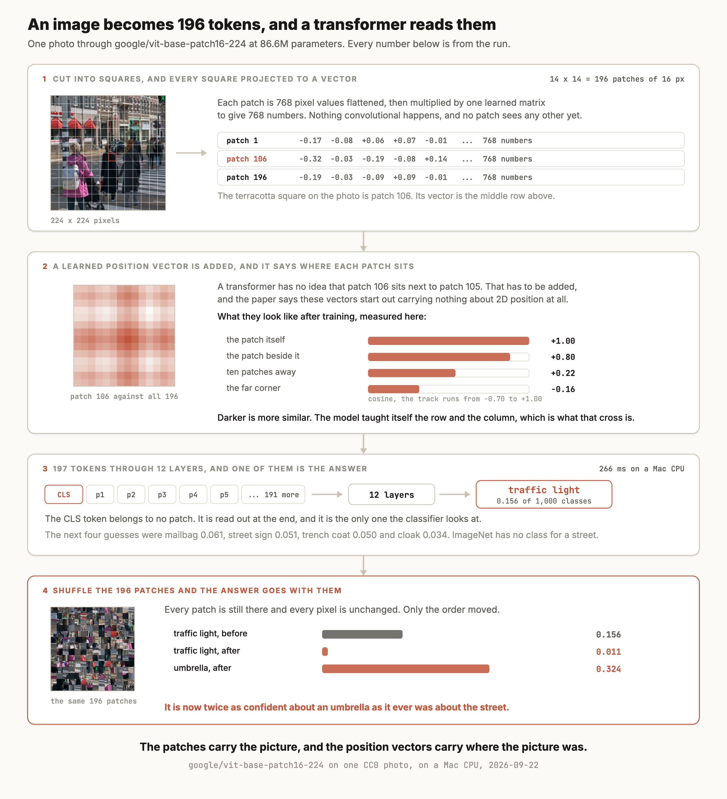
The patch embedding is one matrix multiplication and nothing else, with no convolution and no pooling. The layout inside a patch survives, because every patch is flattened in the same pixel order, so the matrix can learn edge and texture patterns within those 16 by 16 pixels. The paper found its learned filters "resemble plausible basis functions for a low-dimensional representation of the fine structure within each patch". What the embedding can't tell is where a patch sits among the others, for example that patch 92 is directly above patch 106. That arrangement comes from the position vectors added in step two.
Those position vectors are learned, and the paper is explicit that they start out knowing nothing, saying "the position embeddings at initialization time carry no information about the 2D positions of the patches and all spatial relations between the patches have to be learned from scratch". What they look like afterwards is the heatmap: a patch is most similar to itself, then to its neighbours, with a cross along its own row and column. The model worked out the shape of a grid from photographs.
The shuffle in step four shows the model uses that arrangement. Every pixel is still present and only the order of the patches changed, and the answer went from a traffic light at 0.156 to an umbrella at 0.324. The drop shows that the model reads the arrangement of the patches, and a CNN given the same shuffled photo would likely lose its answer too.
Where it shows up
Where Vision Transformers show up
As the eyes of a vision-language model
Every VLM on this index has a ViT in front of the language model. The image-to-tokens step that article describes is this architecture, and the patches it produces become tokens in the prompt.
As the image tower of CLIP and SigLIP
CLIP and SigLIP are two towers, and the image one is a ViT. The most-downloaded Vision Transformer on Hugging Face is not sold as a Vision Transformer at all, it is openai/clip-vit-base-patch32.
As a general-purpose feature extractor
DINOv2 trains a ViT without labels and produces patch features that transfer to segmentation, depth and retrieval. It is the default backbone when you want image features and have no labels to fine-tune with.
Image classification, where it replaced the CNN
Give it a labelled dataset and a classification head and it does the job ResNets did, which is what the original paper set out to show.
Document retrieval over page images
ColPali runs a ViT over a rendered page and keeps one vector per patch. The patches are parts of a document rather than parts of a photograph, and the architecture does not care.
How it works
Patches, positions, and heads that behave like convolutions
Three steps before any attention happens
The image is resized to a fixed size, 224 by 224 in the checkpoint measured here. It is cut into a grid of squares, 14 by 14 of them at 16 pixels each. Each square's pixels are flattened into a list of 768 numbers and multiplied by one learned matrix, giving a vector of 768 numbers per patch.
A learned position vector is then added to each one, and a single extra vector called the CLS token is put at the front. That token belongs to no patch and exists so the model has a slot to accumulate a summary in, the same way BERT uses one.
From there it is an ordinary transformer. Every token attends to every other token at every layer, and after the last layer the CLS token is what the classifier reads.
Attention distance, which is where the difference from a CNN shows
A convolution in the first layer can only see a small square around each pixel, and its view grows one layer at a time. A transformer can look anywhere from the first layer. Whether it actually does is a question you can measure, and the paper measured it with something it calls attention distance, described as "analogous to receptive field size in CNNs".
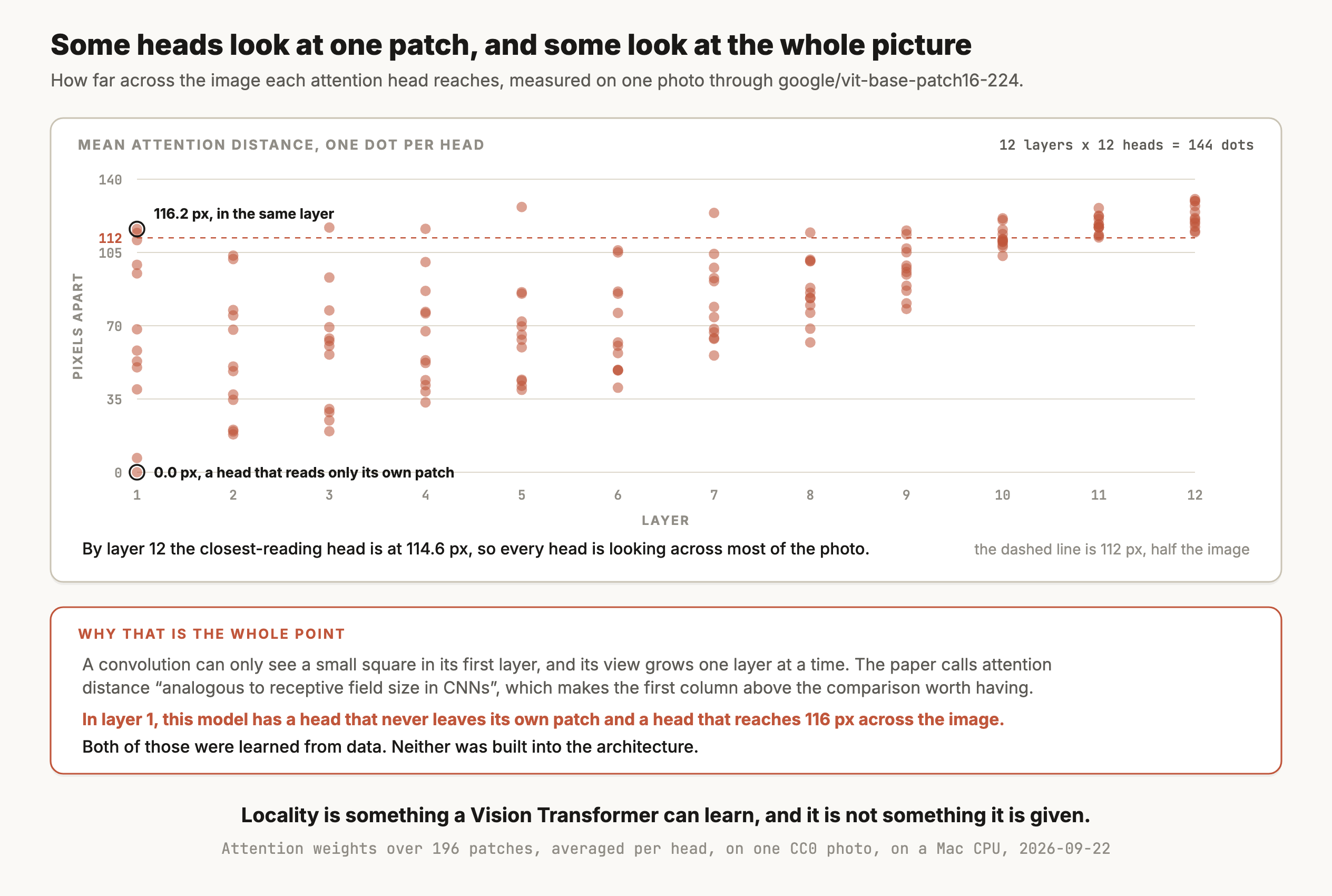
The first layer is the interesting one. One head in it has a mean attention distance of 0.0 pixels, meaning it reads its own patch and nothing else, which is the most local thing a head can do. Another head in the same layer reaches 116.2 pixels, which is more than half the width of the image. The paper found the same split and wrote that "some heads attend to most of the image already in the lowest layers" while others "have consistently small attention distances in the low layers".
By layer 12 the spread is gone and every head sits between 114.6 and 130.5 pixels. Depth pushes everything global.
It needs more data than a CNN, and that was the original problem
A convolution has locality and translation equivariance built into every layer, so it starts out already assuming useful things about images. A ViT assumes far less. Its feed-forward layers work on one patch at a time, and the paper says the two-dimensional layout "is used very sparingly", once when the image is cut into patches and again when position embeddings are resized for a new resolution. The attention layers have no notion of neighbours at all, which is why the paper says transformers "lack some of the inductive biases inherent to CNNs, such as translation equivariance and locality, and therefore do not generalize well when trained on insufficient amounts of data".
Trained on ImageNet alone, the first ViTs came in below ResNets of the same size. Pre-trained on the 14 million images of ImageNet-21k, ViT-L/16 reached 85.30% on ImageNet. The clear win came with Google's in-house JFT-300M dataset, where ViT-H/14 reached 88.55% against 87.54% for BiT-L, a ResNet pre-trained on the same data. The paper sums it up as "large scale training trumps inductive bias".
A later paper narrowed that gap from the training side. DeiT (Touvron et al., 2020) trained an 86M-parameter ViT on ImageNet alone with heavy augmentation and regularization, and reported 83.1% top-1 "with no external data". So a ViT on a mid-sized dataset can work, as long as the training recipe supplies what the architecture doesn't.
That is why almost nobody trains one from scratch. You start from a checkpoint someone pre-trained at that scale, and the BERT article makes the same argument for text.
Resolution and cost are the same dial
Doubling the side of the image quadruples the number of patches, and attention cost grows faster than linearly in the number of tokens. A 16-pixel patch on a 224-pixel image gives 196 tokens, and the same patch size on a 448-pixel image gives 784. The VLM article measures what that costs in a prompt, where a single photo through Qwen2.5-VL arrived as 3,588 tokens.
Fine-tuning at a higher resolution than the checkpoint was trained at means the position embeddings no longer line up, and they get interpolated onto the new grid. That step is standard and it is worth knowing it happened when accuracy moves for no visible reason.
Versions
The checkpoints you'll see, as of September 2026
| Model | Released | License | Downloads a month |
|---|---|---|---|
openai/clip-vit-base-patch32 | March 2022 | Check the card | 22.07M |
google/vit-base-patch16-224 | March 2022 | Apache-2.0 | 7.51M |
facebook/dinov2-base | July 2023 | Apache-2.0 | 3.00M |
google/vit-base-patch16-224-in21k | March 2022 | Apache-2.0 | 1.85M |
timm/vit_base_patch16_224.augreg2_in21k_ft_in1k | December 2022 | Apache-2.0 | 0.45M |
microsoft/resnet-50, the CNN it replaced | March 2022 | Apache-2.0 | 0.56M |
The top row is the point of the table. The most-downloaded Vision Transformer is the image tower of CLIP, pulled three times as often as the original ViT checkpoint, because most people reach for this architecture inside something else.
vit-base-patch16-224 is the checkpoint to read the code of and the one this article measured. The -in21k variant is the same model without the ImageNet-1k classification head, which is what you want when you are fine-tuning on your own labels.
dinov2-base is the one to start from for features. It is the same architecture trained without labels, and the DINO article covers what that changes.
Choosing
Choosing, and when a CNN is still the answer
| The job | Reach for | Why |
|---|---|---|
| Image features, with no labels of your own | DINOv2 | Self-supervised, and its patch features transfer without fine-tuning |
| Classifying into your own labels | vit-base-patch16-224-in21k plus a head | Pre-trained at scale, and the head is the only new part |
| Matching images against text | CLIP or SigLIP | Two towers trained together, which is a different objective from this one |
| Feeding images to a language model | A VLM | The ViT is already inside it, with a projector on top |
| Searching documents as page images | ColPali | Same backbone, one vector kept per patch |
| A small labelled dataset and no pre-training budget | A CNN, or a pre-trained ViT | A from-scratch ViT underperforms here, which the paper measured |
| Real-time detection on a device | YOLO | Built for latency, where this is built for transfer |
| Very high resolution inputs | A hierarchical backbone such as Swin, or a CNN | Patch count and attention cost both grow fast |
Start from a pre-trained checkpoint in every case. In the original paper ViT pulled clearly ahead of a ResNet only with JFT-300M pre-training, and a checkpoint lets you inherit that pre-training without paying for it.
Try it
How to try it
Classifying one image is four lines, and the interesting part is what you can read out of the model while you do it.
import torch
from PIL import Image
from transformers import ViTForImageClassification, ViTImageProcessor

mid = "google/vit-base-patch16-224"                  # 86.6M, Apache-2.0
proc = ViTImageProcessor.from_pretrained(mid)
model = ViTForImageClassification.from_pretrained(mid).eval()

px = proc(images=Image.open("photo.jpg"), return_tensors="pt").pixel_values
with torch.no_grad():
    probs = model(px).logits.softmax(-1)[0]
top = probs.topk(5)
for p, i in zip(top.values, top.indices):
    print(round(float(p), 3), model.config.id2label[int(i)])
Reading the position embeddings takes one more line, and it is the fastest way to convince yourself the grid was learned.
pe = model.vit.embeddings.position_embeddings[0, 1:]   # drop CLS, 196 x 768
pe = torch.nn.functional.normalize(pe, dim=-1)
sim = (pe @ pe.T).detach()

probe = 7 * 14 + 7                        # the patch at row 7, column 7
grid = sim[probe].reshape(14, 14)
print(round(float(grid[7, 7]), 2),        # itself
      round(float(grid[7, 8]), 2),        # the patch beside it
round(float(grid[0, 0]), 2)) # the far cornerShow me what a Vision Transformer has actually learned about space, on my own images. Load google/vit-base-patch16-224 and run it on a folder of photos with output_attentions turned on. For each photo, report the top five predicted labels with probabilities, and compute the mean attention distance for every head in every layer by weighting each patch pair's attention by the distance between their centres in pixels, then plot those 144 numbers as a scatter of distance against layer. Separately, take the learned position embeddings, drop the CLS row, and print the cosine between one patch and every other as a 14 by 14 grid so I can see the row and column structure. Finally, shuffle the 196 patches of each photo in pixel space with a fixed seed, run it again, and report how far the original top label's probability fell.
Limits
What it can't do
- It needs a lot of pre-training, or a heavy training recipe. With the original recipe on ImageNet alone it lands below a comparable ResNet, which the paper states plainly. DeiT closed that gap with augmentation and regularization, and most of what's good about it still arrives with the checkpoint.
- Where each patch sits comes only from learned position vectors. Those vectors are tied to the grid the checkpoint was trained on, so changing input resolution means interpolating them onto a new grid, and accuracy can move when you do.
- Cost grows fast with resolution. Patches scale with area and attention scales worse than linearly with tokens, which is why high-resolution work usually reaches for a hierarchical backbone.
- The output is a label or a set of vectors, and not a location. Boxes and masks need a detection or segmentation head on top, and YOLO exists for the case where latency matters.
- It only sees what fits in the input square. A 224-pixel resize throws away detail, so small text and fine structure are gone before the first layer. That is one of the reasons ColPali runs at page resolution.
- This run is one photo on one checkpoint. It shows the mechanism and the attention spread, and the paper's own figure is the version measured across a dataset.
Go deeper
Dosovitskiy et al. (2020): An Image is Worth 16x16 Words, the ViT paper · Vaswani et al. (2017): Attention Is All You Need, the architecture it reuses · Touvron et al. (2020): DeiT, training a ViT on ImageNet alone · Oquab et al. (2023): DINOv2, the self-supervised ViT most people now use as a backbone
Coming soon
New modules go live as I write them. Get each one in your inbox the day it ships. No spam, just the next lesson.